Loguniform Distribution

Overview

The loguniform distribution (also called the reciprocal distribution) is a two-parameter distribution. This distribution has a probability density function that is proportional to the reciprocal of the variable value within its two bounding parameters (lower and upper limits of its support).

Create a probability distribution object LoguniformDistribution by specifying parameter values (makedist). Then, use object functions to evaluate the distribution, generate random numbers, and so on.

Parameters

The loguniform distribution uses the following parameters.

Parameter	Description	Support
a	Lower limit	0 < a < b
b	Upper limit	a < b < ∞

Probability Density Function

The probability density function (pdf) of the loguniform distribution is

$$f(x|a,b)=\{\begin{array}{c}\left(\frac{1}{x*\log \left(\frac{b}{a}\right)}\right);0<a\le x\le b\\ 0;otherwise\end{array}.$$

For an example, see Compute and Plot Loguniform Distribution pdf.

Cumulative Distribution Function

The cumulative distribution function (cdf) of the loguniform distribution is

$$F\left(x|a,b\right)=\{\begin{array}{c}0;x<a\\ \frac{\log \left(\raisebox{1ex}{$x$}\!\left/ \!\raisebox{-1ex}{$a$}\right.\right)}{\log \left(\raisebox{1ex}{$b$}\!\left/ \!\raisebox{-1ex}{$a$}\right.\right)};a\le x<b\\ 1;x\ge b\end{array}.$$

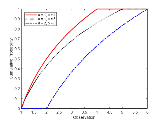
The result p is the probability that a single observation from a loguniform distribution with parameters a and b falls in the interval [a x].

For an example, see Compute Loguniform Distribution cdf.

Descriptive Statistics

The mean of the loguniform distribution is $$\mu =\frac{b-a}{\log \left(\frac{b}{a}\right)}$$.

The variance of the loguniform distribution is $${\sigma }^2=\frac{\log \left(\frac{b}{a}\right)\left(b^2-a^2\right)-2{\left(b-a\right)}^2}{2{\left[\log \left(\frac{b}{a}\right)\right]}^2}$$.

Examples

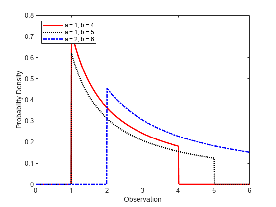
Compute and Plot Loguniform Distribution pdf

Create three loguniform distribution objects with different parameters.

pd1 = makedist('Loguniform')   % Loguniform distribution with default parameters a = 1 and b = 4

pd1 = 
  LoguniformDistribution

  Loguniform distribution
    Lower = 1
    Upper = 4

pd2 = makedist('Loguniform','lower',1,'upper',5); % Loguniform distribution with a = 1 and b = 5
pd3 = makedist('Loguniform','lower',2,'upper',6); % Loguniform distribution with a = 2 and b = 6

Compute the pdfs for the three loguniform distributions.

x = 0:.01:6;
pdf1 = pdf(pd1,x);
pdf2 = pdf(pd2,x);
pdf3 = pdf(pd3,x);

Plot the pdfs on the same axis.

figure;
plot(x,pdf1,'r','LineWidth',2); 
hold on;
plot(x,pdf2,'k:','LineWidth',2);
plot(x,pdf3,'b-.','LineWidth',2);
legend({'a = 1, b = 4','a = 1, b = 5','a = 2, b = 6'},'Location','northwest');
xlabel('Observation')
ylabel('Probability Density')
hold off;

The distribution density is proportional to the reciprocal of the variable value within a and b, hence, the pdf value decreases as the value of the variable increases.

Compute Loguniform Distribution cdf

Create three loguniform distribution objects with different parameters.

pd1 = makedist('Loguniform');  % Loguniform distribution with default parameters a = 1 and b = 4
pd2 = makedist('Loguniform','lower',1,'upper',5); % Loguniform distribution with a = 1 and b = 5
pd3 = makedist('Loguniform','lower',2,'upper',6); % Loguniform distribution with a = 2 and b = 6

Compute the cdfs for the three loguniform distributions.

x = 1:.01:6;
cdf1 = cdf(pd1,x);
cdf2 = cdf(pd2,x);
cdf3 = cdf(pd3,x);

Plot the cdfs on the same axis.

figure;
plot(x,cdf1,'r','LineWidth',2); 
hold on;
plot(x,cdf2,'k:','LineWidth',2);
plot(x,cdf3,'b-.','LineWidth',2);
legend({'a = 1, b = 4','a = 1, b = 5','a = 2, b = 6'},'Location','NW');
xlabel('Observation')
ylabel('Cumulative Probability')
hold off;

Transform Standard Uniform Sample to Loguniform Sample

Create a standard uniformly distributed sample of size 30.

 p = random('Uniform',0,1,30,1);

Compute the loguniform sample with support (2,7) corresponding to the standard uniform values in p.

logunifval = icdf('Loguniform',p,2,7);

Alternatively, first create a loguniform distribution object with support (2,7) and then use it in the call to icdf.

logunifpd = makedist('Loguniform', "Lower",2,"Upper",7)

logunifpd = 
  LoguniformDistribution

  Loguniform distribution
    Lower = 2
    Upper = 7

logunifval2 = icdf(logunifpd,p);

Generate Random Numbers from Loguniform Distribution

To generate random numbers from a loguniform distribution, you must first create a loguniform distribution object. Create a loguniform distribution object with support (3,10).

pd = makedist("Loguniform",3,10)

pd = 
  LoguniformDistribution

  Loguniform distribution
    Lower =  3
    Upper = 10

Generate a 3-by-4 matrix of random numbers from the loguniform distribution.

R = random(pd,3,4)

R = 3×4

    8.0006    9.0096    4.1951    9.5861
    8.9277    6.4235    5.7953    3.6269
    3.4956    3.3738    9.5013    9.6521

Related Distributions

• Uniform Distribution — The continuous uniform distribution is a two-parameter distribution that has parameters a (lower limit) and b (upper limit). If X has a loguniform distribution within the support a and b, then log(X) has a uniform distribution between log(a) and log(b).