Batch Linearize Model for Parameter Value Variations Using Model Linearizer
This example shows how to use the Model Linearizer to batch linearize a Simulink® model. You vary model parameter values and obtain multiple open-loop and closed-loop transfer functions from the model.
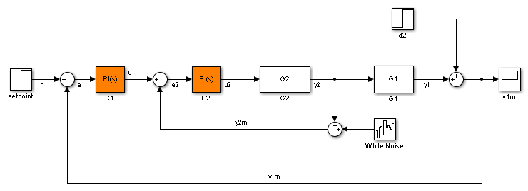
The scdcascade model used for this example contains a pair of
cascaded feedback control loops. Each loop includes a PI controller. The plant models,
G1 (outer loop) and G2 (inner loop), are LTI models. In
this example, you use Model Linearizer to vary the PI controller parameters
and analyze the inner-loop and outer-loop dynamics.
Open Model Linearizer for the Model
At the MATLAB® command line, open the Simulink model.
openExample("scdcascade")To open the Model Linearizer, in the Simulink model window, in the Apps gallery, click Model Linearizer.
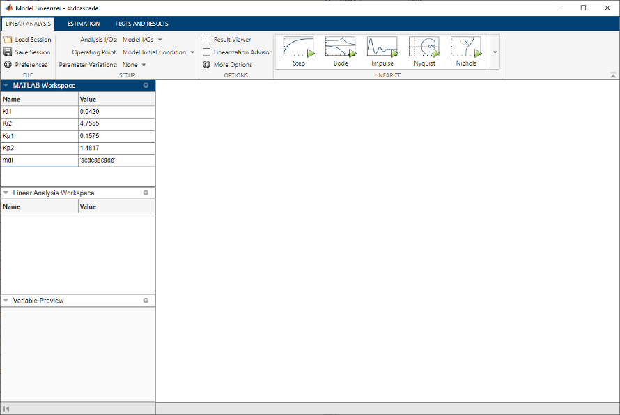
Vary the Inner-Loop Controller Gains
To analyze the behavior of the inner loop, very the gains of the inner-loop PI
controller, C2. As you can see by inspecting the controller block,
the proportional gain is the variable Kp2, and the integral gain
is Ki2. Examine the performance of the inner loop for two
different values of each of these gains.
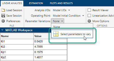
In the Parameter Variations drop-down list, click
![]()
Select parameters to vary.
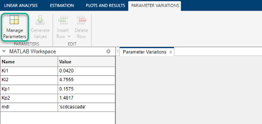
The Parameter Variations tab opens. click
![]() Manage Parameters.
Manage Parameters.
In the Select model variables dialog box, check the parameters to vary,
Ki2 and Kp2.
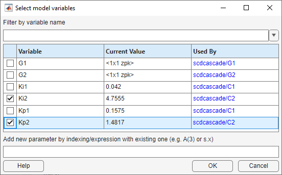
Click OK.
The selected variables appear in the Parameter Variations
table. Each column in the table corresponds to one of the selected variables. Each
row in the table represents one (Ki2,Kp2) pair at which to
linearize the model. These parameter-value combinations are called
parameter samples. When you linearize, Model
Linearizer computes as many linear models as there are parameter samples, or
rows in the table.
Specify the parameter samples at which to linearize the model. For this example,
specify four (Ki2,Kp2) pairs, (Ki2,Kp2) =
(3.5,1), (3.5,2), (5,1), and (5,2). Enter these values in the table manually. To do
so, select a row in the table. Then, select Insert Row > Insert Row Below twice.

Edit the values in the table as shown to specify the four
(Ki2,Kp2) pairs.

Tip
For more details about specifying parameter values, see Specify Parameter Samples for Batch Linearization
Analyze the Inner Loop Closed-Loop Response
To analyze the inner-loop performance, extract a transfer function from the
inner-loop input u1 to the inner-plant output
y2, computed with the outer loop open. To specify this I/O for
linearization, in the Linear Analysis tab, in the
Analysis I/Os drop-down list, select Create New
Linearization I/Os.
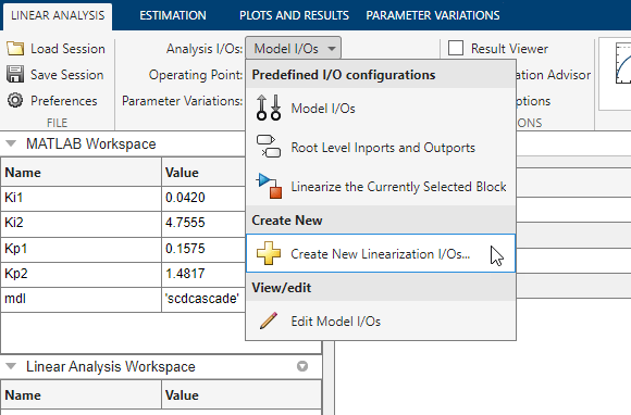
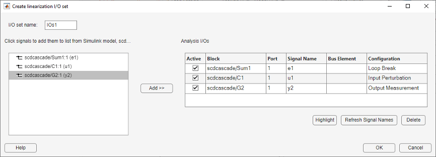
Specify the I/O set by creating:
An input perturbation point at
u1An output measurement point at
y2A loop break at
e1
Name the I/O set by typing InnerLoop in the Variable
name field of the Create linearization I/O set dialog box. The
configuration of the dialog box is as shown.
Tip
For more information about specifying linearization I/Os, see Specify Portion of Model to Linearize.
Click OK.
Now that you have specified the parameter variations and the analysis I/O set for
the inner loop, linearize the model and examine a step response plot. Click
![]() Step.
Step.
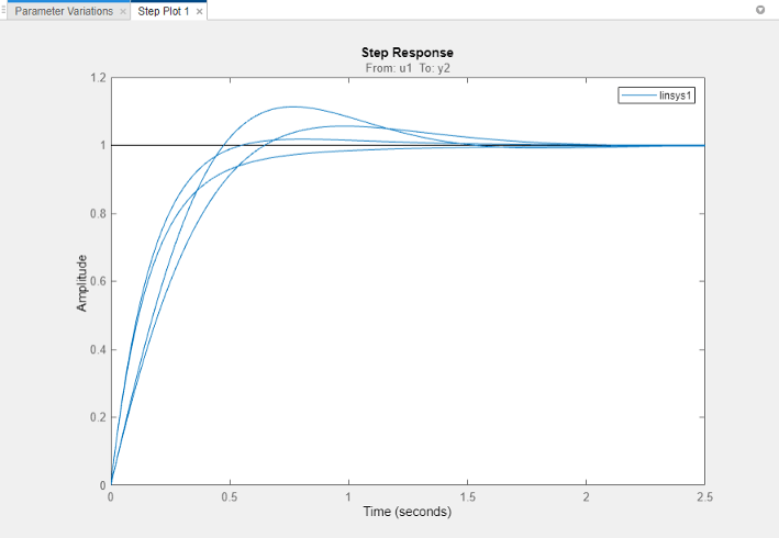
Model Linearizer linearizes the model at each of the parameter samples
you specified in the Parameter Variations table. A new variable,
linsys1, appears in the Linear Analysis Workspace section of
the Data Browser. This variable is an array of state-space (ss)
models, one for each (Ki2,Kp2) pair. The plot shows the step
responses of all the entries in linsys1. This plot gives you a
sense of the range of step responses of the system in the operating ranges covered by
the parameter grid.
Vary the Outer-Loop Controller Gains
Examine the overall performance of the cascaded control system for varying values
of the outer-loop controller, C1. To do so, vary the coefficients
Ki1 and Kp1, while keeping
Ki2 and Kp2 fixed at the values specified in
the model.
In the Parameter Variations tab, click
![]() Manage Parameters. Clear the
Manage Parameters. Clear the Ki2 and
Kp2 checkboxes, and check Ki1 and
Kp1. Click OK.

Use Model Linearizer to generate parameter values automatically. Click
![]() Generate Values. In the Values column of
the Starting Values table, enter an expression specifying the
possible values for each parameter. For example, vary
Generate Values. In the Values column of
the Starting Values table, enter an expression specifying the
possible values for each parameter. For example, vary Kp1 and
Ki1 by ± 50% of their nominal values, by entering
expressions as shown.
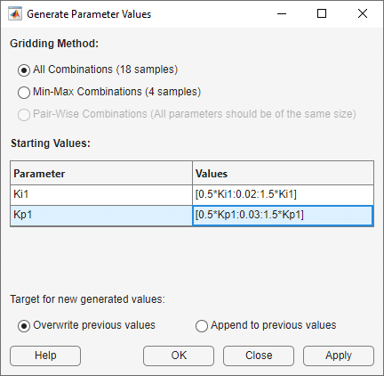
The All Combinations gridding method generates a complete
parameter grid of (Kp1,Ki1) pairs, to compute a linearization at
all possible combinations of the specified values. To replace all values in the
Parameter Variations table with the generated values, elect
Overwrite previous values and click
OK.
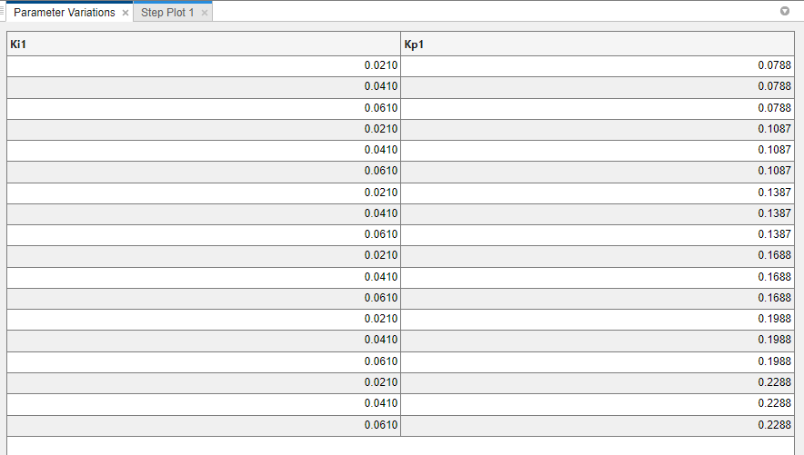
Because you want to examine the overall closed-loop transfer function of the
system, create a new linearization I/O set. In the Linear
Analysis tab, in the Analysis I/Os drop-down list,
select Create New Linearization I/Os. Configure
r as an input perturbation point, and the system output
y1m as an output measurement. Click
OK.
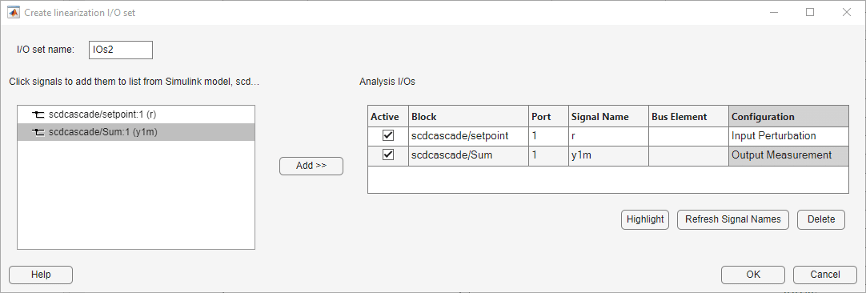
Linearize the model with the parameter variations and examine the step response of
the resulting models. Click ![]() Step to linearize and generate a new plot for the new model
array,
Step to linearize and generate a new plot for the new model
array, linsys2.
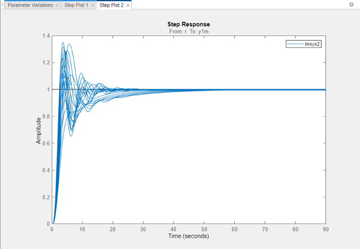
The step plot shows the responses of every model in the array. This plot gives you a sense of the range of step responses of the system in the operating ranges covered by the parameter grid.
Note
Although the new plot reflects the new set of parameter variations,
Step Plot 1 and linsys1 are unchanged.
That plot and array still reflect the linearizations obtained with the inner-loop
parameter variations.
Further Analysis of Batch Linearization Results
The results of both batch linearizations, linsys1 and
linsys2, are arrays of state-space (ss)
models. Use these arrays for further analysis in any of several ways:
Create additional analysis plots, such as Bode plots or impulse response plots, as described in Analyze Results Using Model Linearizer Response Plots.
Examine individual responses in analysis plots as described in Analyze Batch Linearization Results in Model Linearizer.
Export the model arrays to the MATLAB workspace by right-clicking
linsys1orlinsys2in the Linear Analysis Workspace and selecting Export to MATLAB Workspace.You can then use Control System Toolbox™ control design tools, such as the Linear System Analyzer app, to analyze linearization results. Or, use Control System Toolbox control design tools, such as
pidtuneor Control System Designer, to design controllers for the linearized systems.Export your batch linearization results as an LPV model. To do so:
Before linearization, on the Linear Analysis tab, select Prepare for LTV/LPV.
After linearization, on the Plots and Results tab, click Export as LTV/LPV.
Also see Validate Batch Linearization Results for information about validating linearization results in the MATLAB workspace.