Analyze Batch Linearization Results in Model Linearizer
This example shows how to use response plots to analyze batch linearization results in Model Linearizer. The term batch linearization results refers to linearizations for varying parameter values, such as illustrated in Batch Linearize Model for Parameter Value Variations Using Model Linearizer. You can use the techniques illustrated in this example to analyze the frequency response, stability, and other system characteristics for batch linearization results.
View Parameters of a Response
For this example, suppose that you have batch linearized a model as described in
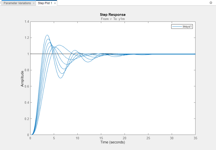
Batch Linearize Model for Parameter Value Variations Using Model Linearizer. You have generated a step response plot of an array of linear models computed for
a 2-D parameter grid, with variations of outer-loop controller gains
Ki1 and Kp1.
When you perform batch linearization, Model Linearizer generates a plot showing the responses of all linear models resulting from the linearization. You choose the response plot type, such as Step, Bode, or Nyquist, when you linearize. You can create additional plots at any time as described in Analyze Results Using Model Linearizer Response Plots.
To view the parameters associated with a particular response, click the response on the plot.
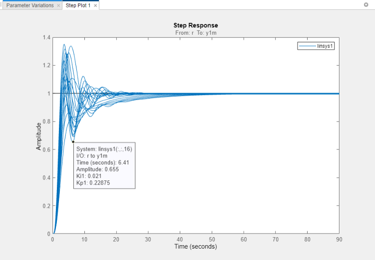
A data tip appears on the plot, providing information about the selected response
and the related model. The last lines of the data tip show the parameter combination
that yielded this response. For example, in this plot, the selected response
corresponds to the model obtained by setting Kp1 to
0.22875 and Ki1 to
0.021.
View Step Response of Subset of Results
Suppose you want to view the responses for only the models linearized at a
specific Ki1 value, the middle value Ki1 =
0.0410. Right-click the plot and select Array
Selector.
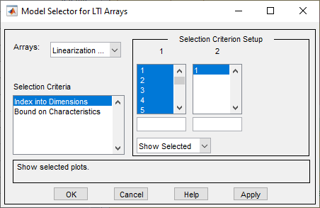
In the Model Selector for LTI Arrays dialog box, the Selection Criterion
Setup section contains two columns, one for each model array dimension
of linsys1. Model Linearizer flattens the 2-D parameter
grid into a one-dimensional array, so that variations in both Kp1
and Ki1 are represented along the indices shown in column
1. To determine which entries in this array correspond to
Ki1 = 0.0410, examine the Parameter
Variations table.
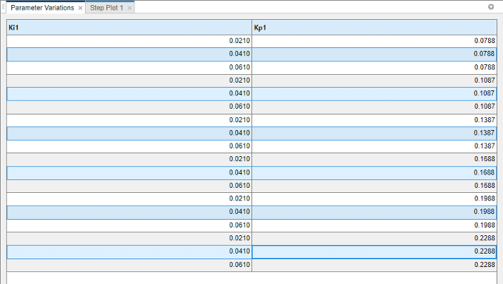
The Ki1 = 0.0410 values are at locations 2, 5, 8, 11, 14, and
17.
In the Model Selector for LTI Arrays dialog box, enter [2 5 8 11 14
17] in the field below column 1. The selection in
the column changes to reflect this subset of the array.
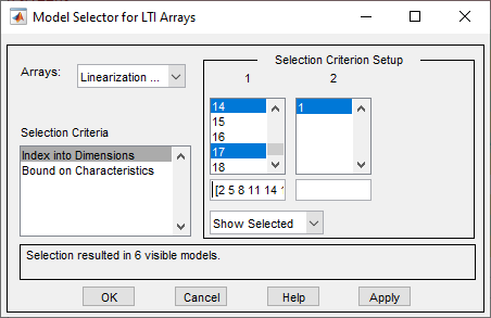
Click OK. The step plot displays responses only for the
models with Ki1 = 0.0410.
Export Array to MATLAB Workspace
You can export the model array to the MATLAB® workspace to perform further analysis or control design. To do so, in the Model Linearizer, in the Linear Analysis Workspace, right click the model array and select Export to MATLAB Workspace.
You can then use Control System Toolbox™ control design tools, such as the Linear System Analyzer app, to analyze
linearization results. Or, use Control System Toolbox control design tools, such as pidtune or Control System Designer, to design controllers for the linearized
systems.