dtw

동적 시간 워핑을 사용한 신호 간 거리

구문

dist = dtw(x,y)

[dist,ix,iy] = dtw(x,y)

[___] = dtw(x,y,maxsamp)

[___] = dtw(___,metric)

dtw(___)

설명

dist = dtw(x,y)는 두 개의 벡터 x와 y를 공통된 순간들의 집합으로 확장하여 이에 대응하는 점 간의 유클리드 거리의 합 dist가 가장 작은 값을 갖도록 합니다. 입력값을 확장하기 위해 dtw는 x와 y의 각 요소를 필요한 횟수만큼 반복합니다. x와 y가 행렬이면 dist는 행렬의 열을 반복하여 이 행렬을 확장합니다. 이 경우, x와 y의 행 개수는 동일해야 합니다.

[dist,ix,iy] = dtw(x,y)는 x(ix)와 y(iy) 간에 가능한 한 가장 작은 dist 값을 가지는 공통된 순간들의 집합, 즉 워핑 경로를 반환합니다.

벡터 ix와 iy의 길이는 같습니다. 각 벡터는 단조 증가하는 시퀀스를 포함합니다. 여기서는 대응되는 신호 x 또는 y의 요소에 대한 인덱스가 필요한 횟수만큼 반복됩니다.

x와 y가 행렬인 경우, ix와 iy는 x(:,ix)와 y(:,iy)가 최소한도로 분리되도록 하는 값을 가집니다.

[___] = dtw(x,y,maxsamp)는 x와 y 간 직선 피팅의 maxsamp개 샘플 내에 있도록 워핑 경로를 제한합니다. 이 구문은 위에 열거된 구문의 출력 인수 중 하나를 반환합니다.

[___] = dtw(___,metric)은 위에 열거된 구문의 입력 인수 중 하나와 함께, 사용할 거리 측정법을 지정합니다.

출력 인수 없이 dtw(___)를 사용하면 원래 신호와 정렬된 신호가 플로팅됩니다.

• 신호가 실수형 벡터이면 함수가 서브플롯에 두 개의 원래 신호를 표시하고 첫 번째 서브플롯 아래의 서브플롯에 정렬된 신호를 표시합니다.

• 신호가 복소수 벡터이면 함수가 원래 신호와 정렬된 신호를 3차원 플롯에 표시합니다.

• 신호가 실수 행렬이면 함수가 imagesc를 사용하여 원래 신호와 정렬된 신호를 표시합니다.

• 신호가 복소수 행렬이면 이 함수는 실수부와 허수부를 각 영상의 상단과 하단에 표시합니다.

예제

처프와 정현파에 대한 동적 시간 워핑

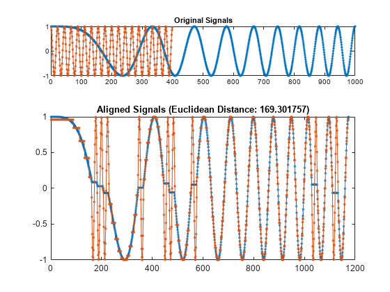
처프와 정현파 각각 하나씩 두 개의 실수 신호를 생성합니다.

x = cos(2*pi*(3*(1:1000)/1000).^2);
y = cos(2*pi*9*(1:399)/400);

점 간의 유클리드 거리 합이 가장 작도록 동적 시간 워핑을 사용하여 신호를 정렬합니다. 정렬된 신호와 거리를 표시합니다.

dtw(x,y);

정현파 주파수를 초기값의 두 배가 되도록 변경합니다. 계산을 반복합니다.

y = cos(2*pi*18*(1:399)/400);

dtw(x,y);

각 신호에 허수부를 추가합니다. 초기 정현파 주파수를 복원합니다. 동적 시간 워핑을 사용하여 유클리드 거리 제곱합을 최소화하는 방식으로 신호를 정렬합니다.

x = exp(2i*pi*(3*(1:1000)/1000).^2);
y = exp(2i*pi*9*(1:399)/400);

dtw(x,y,'squared');

글씨 샘플 정렬하기

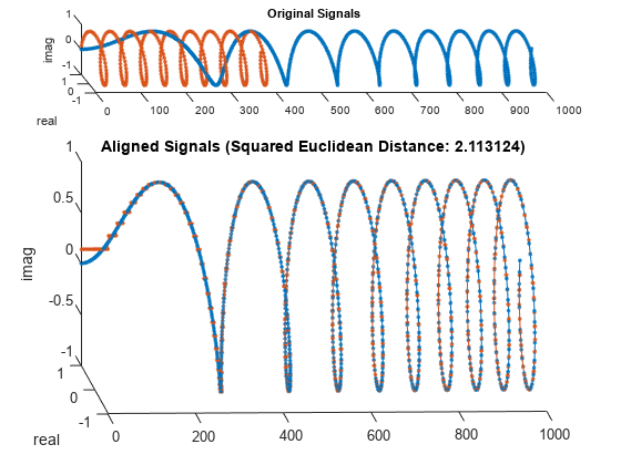
초기 컴퓨터의 출력값과 비슷한 서체를 고안해 보겠습니다. 이를 사용하여 MATLAB®이라는 단어를 씁니다.

chr = @(x)dec2bin(x')-48;

M = chr([34 34 54 42 34 34 34]);
A = chr([08 20 34 34 62 34 34]);
T = chr([62 08 08 08 08 08 08]);
L = chr([32 32 32 32 32 32 62]);
B = chr([60 34 34 60 34 34 60]);

MATLAB = [M A T L A B];

문자로 구성된 난수 열을 반복하고 간격을 다양하게 지정하는 방식으로 단어에 변경을 줍니다. 원래 단어와 세 개의 변경된 형태를 표시합니다. 재현 가능한 결과를 얻기 위해 난수 생성기를 재설정합니다.

rng('default')

c = @(x)x(:,sort([1:6 randi(6,1,3)]));

subplot(4,1,1,'XLim',[0 60])
spy(MATLAB)
xlabel('')
ylabel('Original')

for kj = 2:4
    subplot(4,1,kj,'XLim',[0 60])
    spy([c(M) c(A) c(T) c(L) c(A) c(B)])
    xlabel('')
    ylabel('Corrupted')
end

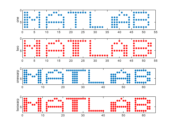
이 단어에 대해 변경된 형태 두 개를 더 생성합니다. 동적 시간 워핑을 사용하여 이 형태들을 정렬합니다.

one = [c(M) c(A) c(T) c(L) c(A) c(B)];
two = [c(M) c(A) c(T) c(L) c(A) c(B)];

[ds,ix,iy] = dtw(one,two);

onewarp = one(:,ix);
twowarp = two(:,iy);

정렬되지 않은 단어와 정렬된 단어를 표시합니다.

figure

subplot(4,1,1)
spy(one)
xlabel('')
ylabel('one')

subplot(4,1,2)
spy(two,'r')
xlabel('')
ylabel('two')

subplot(4,1,3)
spy(onewarp)
xlabel('')
ylabel('onewarp')

subplot(4,1,4)
spy(twowarp,'r')
xlabel('')
ylabel('twowarp')

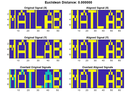
dtw의 내장된 기능을 사용하여 계산을 반복합니다.

dtw(one,two);

제약 조건이 적용된 워핑 경로

길이가 각각 다른 골로 구분된 두 개의 서로 다른 피크로 구성된 두 개의 신호를 생성합니다. 신호를 플로팅합니다.

x1 = [0 1 0 0 0 0 0 0 0 0 0 1 0]*.95;
x2 = [0 1 0 1 0]*.95;

subplot(2,1,1)
plot(x1)
xl = xlim;
subplot(2,1,2)
plot(x2)
xlim(xl)

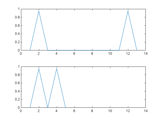
워핑 경로에 제한 없이 신호를 정렬합니다. 완벽하게 정렬하기 위해 이 함수는 더 짧은 신호 샘플 하나만 반복해야 합니다.

figure
dtw(x1,x2);

워핑 경로와 두 신호 간 직선 피팅을 플로팅합니다. 이 함수는 정렬을 위해 피크 사이의 골을 넉넉하게 확장합니다.

[d,i1,i2] = dtw(x1,x2);

figure
plot(i1,i2,'o-',[i1(1) i1(end)],[i2(1) i2(end)])

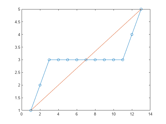
계산을 반복하되, 이번에는 제약 조건을 적용하여 워핑 경로가 직선 피팅에서 3개 요소를 초과해 벗어나지 않도록 합니다. 확장된 신호와 워핑 경로를 플로팅합니다.

[dc,i1c,i2c] = dtw(x1,x2,3);

subplot(2,1,1)
plot([x1(i1c);x2(i2c)]','.-')
title(['Distance: ' num2str(dc)])
subplot(2,1,2)
plot(i1c,i2c,'o-',[i1(1) i1(end)],[i2(1) i2(end)])

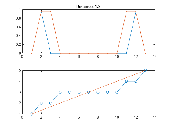
제약 조건을 적용하면 워핑이 샘플의 일부에 너무 많이 집중되지 않도록 합니다. 단, 정렬 품질이 낮아집니다. 단일 샘플 제약 조건을 사용하여 계산을 반복합니다.

dtw(x1,x2,1);

음성 신호에 대한 동적 시간 워핑

$$F_s=7418Hz$$로 샘플링된 음성 신호를 불러옵니다. 이 파일에는 "MATLAB®"이라는 단어를 발음한 여성의 음성이 들어 있습니다.

load mtlb

% To hear, type soundsc(mtlb,Fs)

/æ/ 음소가 발생하는 두 건의 경우에 대응하는 두 세그먼트를 추출합니다. 첫 번째 세그먼트는 대략 150ms에서 250ms 사이에 있고, 두 번째 세그먼트는 370ms에서 450ms 사이에 있습니다. 두 파형을 플로팅합니다.

a1 = mtlb(round(0.15*Fs):round(0.25*Fs));
a2 = mtlb(round(0.37*Fs):round(0.45*Fs));

subplot(2,1,1)
plot((0:numel(a1)-1)/Fs+0.15,a1)
title('a_1')
subplot(2,1,2)
plot((0:numel(a2)-1)/Fs+0.37,a2)
title('a_2')
xlabel('Time (seconds)')

% To hear, type soundsc(a1,Fs), pause(1), soundsc(a2,Fs)

신호 간 유클리드 거리가 최소화되도록 시간 축에 워핑을 적용합니다. 워핑이 적용된 신호에서 공유된 "기간"을 계산하고 플로팅합니다.

[d,i1,i2] = dtw(a1,a2);

a1w = a1(i1);
a2w = a2(i2);

t = (0:numel(i1)-1)/Fs;
duration = t(end)

duration = 
0.1297

subplot(2,1,1)
plot(t,a1w)
title('a_1, Warped')
subplot(2,1,2)
plot(t,a2w)
title('a_2, Warped')
xlabel('Time (seconds)')

% To hear, type soundsc(a1w,Fs), pause(1), sound(a2w,Fs)

하나의 완전한 단어에 대해 같은 실험을 반복합니다. "strong"이라는 단어를 발음한 여성과 남성의 음성이 들어 있는 파일을 불러옵니다. 신호는 8kHz로 샘플링되었습니다.

load('strong.mat')

% To hear, type soundsc(her,fs), pause(2), soundsc(him,fs)

신호 간 절대 거리가 최소화되도록 시간 축에 워핑을 적용합니다. 원래 신호와 변환된 신호를 플로팅합니다. 워핑이 적용된 기간 중에 공유된 "기간"을 계산합니다.

dtw(her,him,'absolute');
legend('her','him')

[d,iher,ihim] = dtw(her,him,'absolute');
duration = numel(iher)/fs

duration = 
0.8394

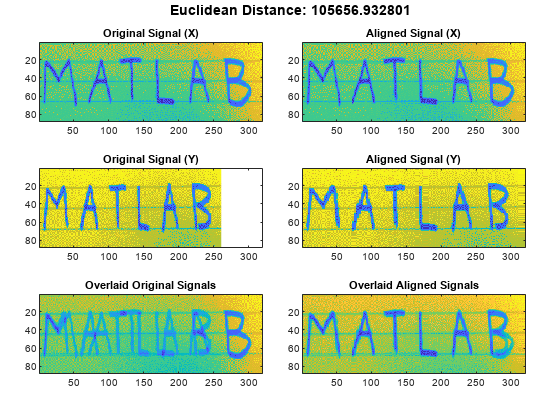
% To hear, type soundsc(her(iher),fs), pause(2), soundsc(him(ihim),fs)

손글씨 정렬을 위한 동적 시간 워핑

파일 MATLAB1.gif와 MATLAB2.gif에는 "MATLAB®"이라는 단어를 손으로 쓴 샘플 두 개가 포함되어 있습니다. 파일을 불러오고 동적 시간 워핑을 사용하여 x축을 따라 정렬합니다.

samp1 = 'MATLAB1.gif';
samp2 = 'MATLAB2.gif';

x = double(imread(samp1));
y = double(imread(samp2));

dtw(x,y);

입력 인수

x — 입력 신호

벡터 | 행렬

입력 신호로, 실수 또는 복소수 벡터나 행렬로 지정됩니다.

데이터형: single | double
복소수 지원 여부: 예

y — 입력 신호

벡터 | 행렬

입력 신호로, 실수 또는 복소수 벡터나 행렬로 지정됩니다.

데이터형: single | double
복소수 지원 여부: 예

maxsamp — 조정 윈도우의 폭

Inf (디폴트 값) | 양의 정수

조정 윈도우의 폭으로, 양의 정수로 지정됩니다.

데이터형: single | double

metric — 거리 측정법

'euclidean' (디폴트 값) | 'absolute' | 'squared' | 'symmkl'

거리 측정법으로, 'euclidean', 'absolute', 'squared' 또는 'symmkl'로 지정됩니다. X와 Y가 모두 K 차원 신호이면 metric은 X의 m 번째 샘플과 Y의 n 번째 샘플 간 거리인 d_mn(X,Y)를 규정합니다. d_mn(X,Y)에 대한 자세한 내용은 동적 시간 워핑 항목을 참조하십시오.

• 'euclidean' — 차이제곱합의 제곱근이며, 유클리드 또는 ℓ₂ 측정법이라고도 합니다.

  $$d_{mn}(X,Y)=\sqrt{{\displaystyle \sum _{k=1}^K{\left(x_{k,m}-y_{k,n}\right)}^{*}\left(x_{k,m}-y_{k,n}\right)}}$$

• 'absolute' — 절대차이합이며, 맨해튼, 도시 블록, 택시 또는 ℓ₁ 측정법이라고도 합니다.

  $$d_{mn}(X,Y)={\displaystyle \sum _{k=1}^K\left|x_{k,m}-y_{k,n}\right|}={\displaystyle \sum _{k=1}^K\sqrt{{\left(x_{k,m}-y_{k,n}\right)}^{*}\left(x_{k,m}-y_{k,n}\right)}}$$

• 'squared' — 유클리드 측정법의 제곱이며, 차이제곱합으로 구성됩니다.

  $$d_{mn}(X,Y)={\displaystyle \sum _{k=1}^K{\left(x_{k,m}-y_{k,n}\right)}^{*}\left(x_{k,m}-y_{k,n}\right)}$$

• 'symmkl' — 대칭적 쿨백-라이블러 측정법(Kullback-Leibler Metric)입니다. 이 측정법은 양의 실수 숫자형 X와 Y에만 유효합니다.

  $$d_{mn}(X,Y)={\displaystyle \sum _{k=1}^K\left(x_{k,m}-y_{k,n}\right)\left(\log x_{k,m}-\log y_{k,n}\right)}$$

출력 인수

dist — 최소 거리

양의 실수형 스칼라

신호 간 최소 거리로, 양의 실수형 스칼라로 반환됩니다.

ix — 첫 번째 신호의 워핑 경로

인덱스 벡터 | 인덱스 행렬

첫 번째 신호의 워핑 경로로, 인덱스 벡터 또는 인덱스 행렬로 반환됩니다.

iy — 두 번째 신호의 워핑 경로

인덱스 벡터 | 인덱스 행렬

두 번째 신호의 워핑 경로로, 인덱스 벡터 또는 인덱스 행렬로 반환됩니다.

세부 정보

동적 시간 워핑

동일한 특징을 가지고 동일한 순서로 정렬된 두 신호라고 해도 각 섹션의 길이가 다르면 매우 다르게 보일 수 있습니다. 동적 시간 워핑은 대응되는 특징이 공통 시간 축에서 같은 위치에 나타나도록 이 기간을 왜곡하여 신호 간 유사성이 두드러지게 합니다.

다음 두 개의 K차원 신호가 있다고 가정해 보겠습니다.

$$X=\left[\begin{array}{cccc}{x}_{1,1}& x_{1,2}& \cdots & x_{1,M}\\ x_{2,1}& x_{2,2}& \cdots & x_{2,M}\\ ⋮& ⋮& \ddots & ⋮\\ x_{K,1}& x_{K,2}& \cdots & x_{K,M}\end{array}\right]$$

및

$$Y=\left[\begin{array}{cccc}{y}_{1,1}& y_{1,2}& \cdots & y_{1,N}\\ y_{2,1}& y_{2,2}& \cdots & y_{2,N}\\ ⋮& ⋮& \ddots & ⋮\\ y_{K,1}& y_{K,2}& \cdots & y_{K,N}\end{array}\right],$$

이 두 신호는 각각 M개 샘플과 N개 샘플을 가집니다. metric에 지정된 X의 m번째 샘플과 Y의 n번째 샘플 간 거리를 나타내는 d_mn(X,Y)가 주어진 경우, dist는 전역 신호 간 거리 측정값이 가장 작도록 X와 Y를 공통된 순간의 집합으로 확장합니다.

처음에, 이 함수는 d_mn(X,Y)의 모든 가능한 값을 다음 형식의 격자로 정렬합니다.

그러면 dist가 길이가 같은 두 시퀀스 ix와 iy로 파라미터화된 격자를 통해 다음이

$$d={\displaystyle \sum _{\begin{array}{c}m\in \text{ix}\\ n\in \text{iy}\end{array}}{d}_{mn}(X,Y)}$$

최소가 되는 경로를 찾습니다. 허용 가능한 dist 경로는 d₁₁(X,Y)에서 시작되고, d_MN(X,Y)에서 종료되며, 체스에서의 킹의 움직임과 같은 다음의 이동이 조합된 형태입니다.

• 수직 이동: (m,n) → (m + 1,n)

• 수평 이동: (m,n) → (m,n + 1)

• 대각선 이동: (m,n) → (m + 1,n + 1)

이 구조에서는 허용 가능한 모든 경로가 전체 신호를 정렬하고, 샘플을 건너뛰지 않고, 신호 특징을 반복하지 않도록 보장됩니다. 또한, 바람직한 경로는 d₁₁(X,Y)와 d_MN(X,Y)를 연결하는 대각선에 가까운 경로입니다. maxsamp 인수로 조정된 이러한 추가 제약 조건을 적용하면 워핑이 유사한 길이의 섹션을 비교하고 이상값 특징을 과적합하지 않게 됩니다.

다음과 같은 격자 통과 경로는 가능합니다.

다음 경로는 허용되지 않습니다.

전체 신호를 정렬하지 않음	샘플을 건너뜀	가던 길을 다시 돌아와서 특징을 반복함

참고 문헌

[1] Paliwal, K. K., Anant Agarwal, and Sarvajit S. Sinha. "A Modification over Sakoe and Chiba’s Dynamic Time Warping Algorithm for Isolated Word Recognition." Signal Processing. Vol. 4, 1982, pp. 329–333.

[2] Sakoe, Hiroaki, and Seibi Chiba. "Dynamic Programming Algorithm Optimization for Spoken Word Recognition." IEEE^® Transactions on Acoustics, Speech, and Signal Processing. Vol. ASSP-26, No. 1, 1978, pp. 43–49.

확장 기능

C/C++ 코드 생성
MATLAB® Coder™를 사용하여 C 코드나 C++ 코드를 생성할 수 있습니다.

버전 내역

R2016a에 개발됨

참고 항목

alignsignals | edr | finddelay | findsignal | xcorr