Calculating an Appropriate BallRadiusConstant for PlannerRRStar

This example explains the BallRadiusConstant of plannerRRTStar in greater detail, and provides intuition on how to calculate a reasonable value for a given planning problem.

What is the BallRadiusConstant?

RRT vs RRT*

The major difference between RRT and RRT* is the "rewiring" behavior, which gives RRT* its asymptotic optimality guarantee. When a new node, ${\mathit{x}}_{\mathrm{new}}$ is generated in RRT-based planners, the planner finds the nearest node in the tree, ${\mathit{x}}_{\mathrm{nearest}}$. If the path between nodes is valid (e.g. collision-free), RRT just connects the nodes, but RRT* performs additional steps to optimize the tree.

First, RRT* finds all nodes in the tree within some distance to ${\mathit{x}}_{\mathrm{new}}$, ${\mathit{X}}_{\mathrm{near}}=\left\{{\mathit{x}}_{\mathit{a}}{\mathit{x}}_{\mathit{b}}...\right\}$. RRT* then finds the node, ${\mathit{x}}^{*}\in {\mathit{X}}_{\mathrm{near}}$, which provides ${\mathit{x}}_{\mathrm{new}}$ with the shortest valid path back to ${\mathit{x}}_{\mathrm{start}}$ and creates an edge between this pair. Lastly, the planner performs a "rewire" operation, which checks whether ${\mathit{x}}_{\mathrm{new}}$ can provide each $\mathit{x}\in {\mathit{X}}_{\mathrm{near}}$ with a shorter route to back to ${\mathit{x}}_{\mathrm{start}}$, in which case $\mathit{x}$ is disconnected from its current parent and reparented to ${\mathit{x}}_{\mathrm{new}}$.

Rewire radius

The goal of RRT* is to provide this asymptotic optimality guarantee while limiting additional overhead. Therefore it is important to choose an appropriately-sized ball-radius during the rewire step - too large and the algorithm's runtime performance will suffer, too small and the algorithm may fail to converge. The distance used by plannerRRTStar to find nearest neighbors is calculated using the following formula adapted from [1]:

(1) $\mathit{r}=\min \left({\left(\gamma *\frac{\log \left(\mathit{N}\right)}{\mathit{N}}\right)}^{\frac{1}{\mathit{d}}},\eta \right),\mathrm{where}$

$$\mathit{N}:\mathit{\#}\mathrm{nodes}\mathrm{in}\mathrm{tree}$$

$$\mathit{d}:\mathit{\#}\mathrm{dimensions}\mathrm{of}\mathrm{the}\mathrm{state}-\mathrm{space}$$

$$\eta :\mathrm{MaxConnectionDistance}$$

$$\gamma :\mathrm{BallRadiusConstant}$$

(2) $\gamma =2^{\mathit{d}}*\left(1+\frac{1}{\mathit{d}}\right)*\frac{\mathrm{vFree}}{\mathrm{vUnitBall}}$

$$\mathrm{vFree}:\mathrm{Lebesgue}\mathrm{Measure}$$

$$\mathrm{vUnitBall}:\mathrm{volume}\mathrm{of}\mathrm{unit}-\mathrm{ball}\mathrm{in}\mathit{d}\mathrm{dimensions}$$

Meaning and intuition behind the BallRadiusConstant

The formulae above define a radius of "appropriate" size for a given space, meaning as the number of nodes filling the space grows linearly, the radius should shrink so that the number of neighbors inside the shrinking ball only grows logarithmically.

The rough intuition here stems from the expectation that all points ${\mathit{x}}_{\mathrm{new}}$$\in \mathit{X}$ in the tree have been uniformly and independently sampled from the free-portion of the configuration space. Points sampled this way can be said to have been generated by a Homogeneous Poisson Point Process.

So for a given iteration of the algorithm, N points have been uniformly sampled in the free space, which means there should be an average density of points per unit volume (or "intensity" of points per unit "measure", for spaces of arbitrary dimensions):

(3) $\lambda =\frac{\mathit{N}}{\mathrm{vFree}}$ = density

It therefore follows that the number of points you can expect to see in any portion of the planning space is just the volume of that portion multiplied by density. For this example, the number of points within a d-ball of radius $\mathit{r}$ is more important:

$$\left(4\right){\mathit{n}}_{1,\mathit{d}}=\mathrm{vUnitBall}*\lambda =\frac{\mathrm{vUnitBall}}{\mathrm{vFree}}*\mathit{N}$$

$$\left(5\right){\mathit{n}}_{\mathit{r},\mathit{d}}={\mathit{n}}_{1,\mathit{d}}*{\mathit{r}}^{\mathit{d}}$$

$${\mathit{n}}_{1,\mathit{d}}:\mathrm{expected}\mathrm{\#points}\mathrm{inside}\mathrm{unit}-\mathrm{ball}$$

$${\mathit{n}}_{\mathit{r},\mathit{d}}:\mathrm{expected}\mathrm{\#points}\mathrm{inside}\mathrm{ball}\mathrm{of}\mathrm{radius}\mathit{r}$$

Recalling that the goal is for the number of neighbors to grow logarithmically as $\mathit{N}\to \infty$, set ${\mathit{n}}_{\mathit{r},\mathit{d}}=\log \left(\mathit{N}\right)$ and solve for $\mathit{r}$:

$$\left(6\right)\mathit{r}={\left(\frac{\mathrm{vFree}}{\mathrm{vUnitBall}}*\frac{\log \left(\mathit{N}\right)}{\mathit{N}}\right)}^{\frac{1}{\mathit{d}}}$$

The remaining coefficients from equation two are derived from the convergence proof in Appendix G of [1], but with $\mathit{N}$ removed. Notice that BallRadiusConstant is only the ratio of free-space in the sample-able region vs the measure of the unit-ball multiplied by a dimension-specific constant.

Visualizing radius vs N and BallRadiusConstant

Now that we've shown the relationship between BallRadiusConstant and the radius, let's view their behavior and see if it matches the intuition:

% Plot unsaturated radius as N increases for different dimensions
figure;
d = [2 3 6 10];
N = logspace(0,6,1000)';
r = (log(N)./N).^(1./d);
legendEntries = "d = " + split(num2str(d));
exampleHelperPlotBallRadius(gca,N,r,"\gamma = 1",legendEntries);

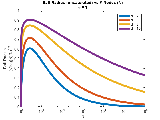
The first thing that stands out is that all radii decay gradually as $\mathit{N}\to \infty$. This aligns with equation (3)/(6), which show the reciprocal relationship between a linearly increasing density and the goal of a logarithmically increasing number of neighbors. The plot also shows how problems in higher dimensions requires a larger radius over a longer period of time, as $\mathit{N}$ points produce a lower density in a higher-dim space than the same number would in a lower-dim space.

% Plot unsaturated radius for 3-dim space with varying BallRadiusConstant
figure;
dIdx = 2;
gammaEstimate = (50:50:250).^(d(dIdx));
rGamma = r(:,d(dIdx)).*(gammaEstimate.^(1/d(dIdx)));
legendEntries = "\gamma= " + split(num2str(gammaEstimate));
exampleHelperPlotBallRadius(gca,N,rGamma,"d = " + num2str(d(dIdx)),legendEntries);

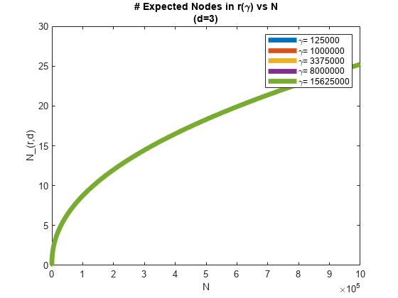
Lastly, plot the number of expected neighbors as $\mathit{N}\to \infty$, for different $\gamma$ against their corresponding $\mathit{r}$ and show that in all cases, the number of expected neighbors at equivalent iterations are identical and increase logarithmically.

% Plot expected number of neighbors as N increases
figure;
nNeighbor = rGamma.^d(dIdx).*(N./log(N))./gammaEstimate./(2^d(dIdx)*(1+1/d(dIdx)));
plot(N,nNeighbor,LineWidth=5);
title(["# Expected Nodes in r(\gamma) vs N","(d=3)"]);
xlabel("N");
ylabel("N\_(r,d)");
legend(legendEntries);

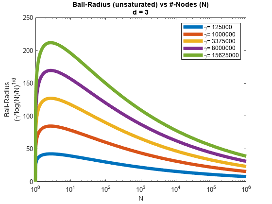
So what happens if the gamma is incorrect? Observe that in the second plot, providing a smaller gamma produces a smaller radius, and since the d-ball is already small when N is small (i.e. the density is low), the likelihood of the ball containing more than a single point becomes very low. More importantly, the number of points you can expect only increases logarithmically by design, so while it is possible that the density eventually catches up to the shrinking volume, you will need to have already processed a large number of points, meaning the effect of a rewiring optimization will be limited to a much smaller portion of the tree.

Effects of an Insufficient BallRadiusConstant

The formulas in What is BallRadiusConstant? shows the approximate lower bound required to achieve the asymptotic guarantee of RRT*'.

Next set up a planning problem where BallRadiusConstant is not large enough to show the planner result.

Set up the planning problem

% Load an occupancyMap
load exampleMaps.mat; 
smallMap = occupancyMap(ternaryMap);
res = smallMap.Resolution;

% Create a state-space whose bounds span the map limits
limits = [smallMap.XWorldLimits; smallMap.YWorldLimits; -pi pi];
ss = stateSpaceSE2(limits);

% Create a state-validator
sv = validatorOccupancyMap(ss,Map=smallMap);
sv.ValidationDistance = (1/res)/10;

% Define start and goal locations
start = [100 100 0]; goal = [400 350 0];

Plan using RRT* with default BallRadiusConstant

% Define RRT* planner with default BallRadiusConstant
maxDist = 20;
rrtStar = plannerRRTStar(ss,sv,MaxConnectionDistance=maxDist,ContinueAfterGoalReached=true);

% Plan a path with RRT*
rng(0);
tic;
[rrtStarPath, rrtStarSolnInfo] = plan(rrtStar,start,goal);
tRRTStarDefault = toc;

Compare results against standard RRT

% Plan path for the same problem using RRT
rrt = plannerRRT(ss,sv,MaxConnectionDistance=maxDist);
rng(0);
[rrtPath, rrtSolnInfo] = plan(rrt,start,goal);

% Display results, note how the RRT* tree fails to optimally explore the
% space.
subplot(1,2,1);
show(smallMap); 
title(["RRT*", "\gamma = 100 (default)"]);
hold on;
plot(rrtStarSolnInfo.TreeData(:,1),rrtStarSolnInfo.TreeData(:,2));
plot(rrtStarPath.States(:,1),rrtStarPath.States(:,2),LineWidth=5);

% Compare these results to the generic RRT planner
subplot(1,2,2);
show(smallMap);
title("RRT");
hold on;
plot(rrtSolnInfo.TreeData(:,1),rrtSolnInfo.TreeData(:,2));
plot(rrtPath.States(:,1),rrtPath.States(:,2),LineWidth=5);
hold off;

When using RRT*, you can expect to see paths that radiate outward from the start state, but instead you see results which are nearly identical to those of RRT. This is an indication that the BallRadiusConstant is poorly adapted to the problem, so next you calculate a more appropriate value.

Calculate Appropriate BallRadiusConstant

Calculate Unit-Ball Volume

To correctly size the constant, you must estimate the Lebesgue Measure of the search space ($\mathrm{vFree})$, and the volume of a unit-ball ($\mathrm{vBall})$ defined in the SE2 space, where states are represented as $\left[\mathit{x}\mathit{y}\theta \right]$:

% Get the number of dimensions in the state-space (SE2 is a 3-dimensional
% state-space)
d = ss.NumStateVariables;

Calculating $\mathrm{vBall}$ is straightforward, handled by exampleHelperNBallVolume:

% Calculate unit-ball volume in d dimensions
vUnitBall = exampleHelperNBallVolume(d);

Approximate Free Volume of the Space

The Lebesgue Measure is a measure of the volume in subsets of an n-dimensional Euclidean space. In layman's terms, this just means the cumulative volume contained within a collection of sub-regions of the space, and in the context of this example, you must find the volume of free-space contained in the search domain.

The occupancyMap provides a discrete representation of the space in XY, with all theta being valid if the corresponding cell is valid. Therefore you can define the volume of a free cell as the area of the cell, multiplied by the max distance between two orientations:

L = 1/res; % Cell length/width
A = L^2;
vCell = A*pi; % Max orientation dist for stateSpaceSE2 is pi

The total free space is the volume of a free cell multiplied by the number of free cells in the search region:

numFreeCells = nnz(checkOccupancy(smallMap) == 0);
vFree = vCell*numFreeCells;

Calculate BallRadiusConstant

Calculate the BallRadiusConstant:

gammaEstimate = (2^d)*(1+1/d)*(vFree/vUnitBall);

Compare RRT* Results Using Appropriate BallRadiusConstant

Plan using the new BallRadiusConstant

% Update the BallRadiusConstant
rrtStar.BallRadiusConstant = gammaEstimate;
rng(0);
tic;
[rrtStarCorrectedPath,rrtStarCorrectedSolnInfo] = plan(rrtStar,start,goal);
tRRTStarCorrected = toc;

Analyze Results

% Display original results
figure
subplot(1,2,1);
show(smallMap);
title(["RRT*","\gamma = 100 (default)"])
hold on;
plot(rrtStarSolnInfo.TreeData(:,1),rrtStarSolnInfo.TreeData(:,2));
plot(rrtStarPath.States(:,1),rrtStarPath.States(:,2),LineWidth=5);

% Display corrected results
subplot(1,2,2);
show(smallMap);
title(["RRT*", "\gamma = " + num2str(gammaEstimate)]);
hold on;
plot(rrtStarCorrectedSolnInfo.TreeData(:,1),rrtStarCorrectedSolnInfo.TreeData(:,2));
plot(rrtStarCorrectedPath.States(:,1),rrtStarCorrectedPath.States(:,2),LineWidth=5);
hold off

Note how the tree built from a properly tuned BallRadiusConstant ($\gamma =1193200$) radiates away from the start state as it expands through the space. Compare this to the default planner whose tree continues to subdivide the space but does not improve the branches.

Verify the improvement to path length by looking at some quantitative results. First load some results obtained offline, where the RRT* planner searched for a path on the same problem using different BallRadiusConstant:

% Generate new results with the following
exampleHelperGenerateOfflineComparison(rrtStar,start,goal,gammaCompared);

% Load offline planning results
load("plannerComparison.mat","t","gammaCompared","pathCosts");

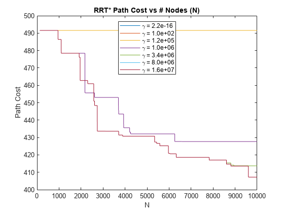
First, compare path lengths returned in the solutionInfo struct as nodes are added to the tree. Note how below a certain $\gamma$value, all planners produce the same results and the path length does not improve after the initial solution is found.

figure;
plot(pathCosts);
title("RRT* Path Cost vs # Nodes (N)");
xlabel("N");
ylabel("Path Cost");
legendEntries = "\gamma = " + num2str(gammaCompared(:),"%3.1e");
legend(legendEntries,Location="north");

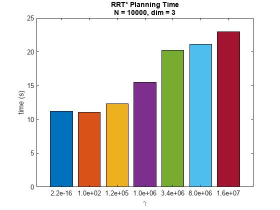
Next, compare time spent during planning. Note that a larger $\gamma$coincides with slower planning performance. This aligns with the expectation that more nodes are being considered per iteration during the rewire step. Note that the increase in computation appears to fall off as $\gamma$continues to grow larger. This likely indicates that the planner is using $\mathit{r}=\eta$(the planner's MaxConnectionDistance) for larger periods during planning, thereby limiting the number of neighbors considered until $\mathit{N}$ grows large enough for $\gamma <\eta$.

% Convert gamma values to categories
x = categorical(string(num2str(gammaCompared(:),"%3.1e")));
x = reordercats(x,string(x));
cOrder = colororder;

% Compare RRT* runtime performance for different gamma
bar(x,t,FaceColor="flat",CData=cOrder(mod(0:numel(x)-1,size(cOrder,1))+1,:));
title(["RRT* Planning Time","N = " + num2str(size(pathCosts,1)) + ", dim = 3"]);
xlabel("\gamma");
ylabel("time (s)");

Summary

This example provided some background on the differences between RRT and RRT* and introduce the concept of the BallRadiusConstant. First the example showed the relationship between the BallRadiusConstant and the rewire radius of RRT*. Additionally, the example showed how this constant impacts planning behavior by changing the average number of neighbors considered during the rewire step.

Next, the example showed how specific terms ($\mathrm{vBall},\mathrm{vFree}$) could be derived from a given planning problem using the state-space dimensionality and the Lebesgue Measure (derived from the occupancyMap). Then the example compared the results produced by RRT* using this more appropriately sized BallRadiusConstant against those generated using the default.

Lastly, the example analyzed a set of offline results for the same problem over a wide range of BallRadiusConstant values and discussed the trends and tradeoffs between planner optimality and computational efficiency.

References

[1] Karaman, Sertac, and Emilio Frazzoli. “Sampling-Based Algorithms for Optimal Motion Planning.” The International Journal of Robotics Research, vol. 30, no. 7, June 2011, pp. 846–94. DOI.org (Crossref), https://doi.org/10.1177/0278364911406761.

[2] S. M. LaValle. Planning Algorithms.Cambridge University Press, 2006.