QP Optimization Problem for Linear MPC
Overview
The classical linear model predictive control solves an optimization problem – specifically, a quadratic program (QP) – at each control interval. The solution determines the manipulated variables (MVs) to be used in the plant until the next control interval. For more information on the QP solvers used to solve the QP problem, see QP Solvers for Linear MPC.
The QP problem includes the following features:
The objective, or "cost", function — A scalar, nonnegative measure of controller performance to be minimized.
Constraints — Conditions the solution must satisfy, such as physical bounds on MVs and plant output variables.
Decision — The MV adjustments that minimize the cost function while satisfying the constraints.
The following sections describe these features in more detail.
Standard Cost Function
The standard cost function is the sum of four terms, each focusing on a particular aspect of controller performance, as follows:
Here, zk is the QP decision. As described below, each term includes weights that help you balance competing objectives. While the MPC controller provides default weights, you will usually need to adjust them to tune the controller for your application.
Output Reference Tracking
In most applications, the controller must keep selected plant outputs at or near specified reference values. An MPC controller uses the following scalar performance measure for output reference tracking:
Here,
k — Current control interval
p — Prediction horizon (number of intervals)
ny — Number of plant output variables
zk — QP decision variables vector, given by:
yj(k+i|k) — Predicted value of the jth plant output at the ith prediction horizon step, in engineering units
rj(k+i|k) — Reference value for the jth plant output at the ith prediction horizon step, in engineering units
— Scale factor for the jth plant output, in engineering units.
— Tuning weight for the jth plant output at the ith prediction horizon step (dimensionless).
εk — Slack variable for constraint softening at control interval k (dimensionless).
The values ny, p, , and are constant controller specifications. The controller receives reference values, rj(k+i|k), for the entire prediction horizon. The controller uses the state observer to predict the plant outputs, yj(k+i|k), which depend on manipulated variable adjustments (zk), measured disturbances (MD), and state estimates. At interval k, the controller state estimates and MD values are available. Therefore, Jy is a function of zk only.
The problem formulation used here, in which the decision variables of the optimization problem are just the manipulated variables (plus a slack variable), is called a dense formulation. it is also known as a sequential or single-shooting formulation.
A different formulation is possible in which the decision variables of the optimization problem also include all the intermediate state variables. In this case, equality constraints of the type x(k+1) = Ax(k) + Bu(k) must be enforced. This formulation results in a larger problem with many equality constraints, but a more regular sparse structure, an easier-to-compute cost function, and better numerical conditioning for large horizons. This alternative formulation is referred to as sparse, (but also simultaneous or multiple-shooting) approach.
The default problem formulation used in Model Predictive Control Toolbox™ for linear MPC problems is the dense formulation, because it can have a smaller memory footprint (if a generic QP solver is used) and tends to be more efficient for stable linear problems in which the prediction horizon is small and when a considerable amount of Manipulated Variable Blocking is used.
Manipulated Variable Tracking
In some applications, such as when there are more manipulated variables than plant outputs, the controller must keep selected manipulated variables (MVs) at or near specified target values. An MPC controller uses the following scalar performance measure for manipulated variable tracking:
Here,
k — Current control interval
p — Prediction horizon (number of intervals)
nu — Number of manipulated variables
zk — QP decision variables vector, given by:
uj,target(k+i|k) — Target value for the jth MV at the ith prediction horizon step, in engineering units
— Scale factor for the jth MV, in engineering units
— Tuning weight for the jth MV at the ith prediction horizon step (dimensionless)
εk — Slack variable for constraint softening at control interval k (dimensionless)
The values nu, p, , and are constant controller specifications. The controller receives uj,target(k+i|k) values for the entire horizon. The controller uses the state observer to predict the plant outputs. Thus, Ju is a function of zk only.
Manipulated Variable Move Suppression
Most applications prefer small MV adjustments (moves). An MPC constant uses the following scalar performance measure for manipulated variable move suppression:
Here,
k — Current control interval
p — Prediction horizon (number of intervals)
nu — Number of manipulated variables
zk — QP decision variables vector, given by:
— Scale factor for the jth MV, in engineering units
— Tuning weight for the jth MV movement at the ith prediction horizon step (dimensionless)
εk — Slack variable for constraint softening at control interval k (dimensionless)
The values nu, p, , and are constant controller specifications. u(k–1|k) = u(k–1), which are the known MVs from the previous control interval. JΔu is a function of zk only.
In addition, a control horizon m < p (or MV blocking) constrains certain MV moves to be zero.
Constraint Violation
In practice, constraint violations might be unavoidable. Soft constraints allow a feasible QP solution under such conditions. An MPC controller employs a dimensionless, nonnegative slack variable for constraint softening, εk, which quantifies the worst-case constraint violation (See Constraints). The corresponding performance measure is:
Here,
zk — QP decision variables vector, given by:
εk — Slack variable for constraint softening at the control interval k (dimensionless).
ρε — Constraint violation penalty weight (dimensionless). This weight corresponds to the
Weights.ECRproperty of anmpcobject.
Alternative Cost Function
You can elect to use the following alternative to the standard cost function:
Here, Q (ny-by-ny), Ru, and RΔu (nu-by-nu) are positive-semi-definite weight matrices, and:
Also,
LSy — Diagonal matrix of plant output variable scale factors sy, in engineering units
LSu — Diagonal matrix of MV scale factors su, in engineering units
r(k+1|k) — ny plant output reference values at the ith prediction horizon step, in engineering units
y(k+1|k) — ny plant outputs at the ith prediction horizon step, in engineering units
zk — QP decision variables vector, given by:
utarget(k+i|k) — nu MV target values corresponding to u(k+i|k), in engineering units.
Output predictions use the state observer, as in the standard cost function.
The alternative cost function allows off-diagonal weighting, but requires the weights to be identical at each prediction horizon step.
The alternative and standard cost functions are identical if the following conditions hold:
The standard cost functions employs weights , , and that are constant with respect to the index, i = 1:p.
The matrices Q, Ru, and RΔu are diagonal with the squares of those weights as the diagonal elements.
Constraints
Certain constraints are implicit. For example, a control horizon m < p (or MV blocking) forces some MV increments to be zero, and the state observer used for plant output prediction is a set of implicit equality constraints. Explicit constraints that you can configure are described below.
Bounds on Plant Outputs, MVs, and MV Increments
The most common MPC constraints are bounds, as follows.
Here, the V parameters (ECR values) are dimensionless controller
constants analogous to the cost function weights but used for constraint softening, and
correspond to the MinECR, MaxECR,
RateMinECR and RateMaxECR vectors stored in
the OutputVariables and ManipulatedVariables
properties of an mpc object. For more information, see Specify Constraints.
Also,
εk — Scalar QP slack variable for constraint softening (dimensionless).
— Scale factor for jth plant output, in engineering units.
— Scale factor for jth MV, in engineering units.
yj,min(i), yj,max(i) — lower and upper bounds for jth plant output at ith prediction horizon step, in engineering units.
uj,min(i), uj,max(i) — lower and upper bounds for jth MV at ith prediction horizon step, in engineering units.
Δuj,min(i), Δuj,max(i) — lower and upper bounds for jth MV increment at ith prediction horizon step, in engineering units.
Except for the slack variable non-negativity condition, all of the above constraints are optional and are inactive by default (i.e., initialized with infinite limiting values). To include a bound constraint, you must specify a finite limit when you design the controller.
Mixed Input/Output Linear Constraints
You can also introduce mixed input/output linear constraints.
The general form of the mixed input/output constraints is:
Eu(k + j) + Fy(k + j) + Sv(k + j) ≤ G + εV
Here, j = 0, ...,p, and:
p is the prediction horizon.
k is the current time index.
u is a column vector manipulated variables.
y is a column vector of all plant output variables.
v is a column vector of measured disturbance variables.
ε is a scalar slack variable used for constraint softening (as in Standard Cost Function).
E, F, G, V, and S are constant matrices.
For more information, see Constraints on Linear Combinations of Inputs and Outputs, setconstraint, getconstraint and Update Mixed Input/Output Constraints at Run Time.
QP Matrices
This section describes the matrices associated with the model predictive control optimization problem described in QP Optimization Problem for Linear MPC. Note that the vector of decision variables used in this section (and in the actual implementation of the software) is:
where
This vector of decision variables is mathematically equivalent to the one described in the previous sections, but, from an implementation perspective, has advantages for formulations that allow for weights and constraints on increments of manipulated variables.
Prediction
Assume that the disturbance models described in Input Disturbance Model are unit gains; that is, d(k) = nd(k) is white Gaussian noise. You can denote this problem as
Then, the prediction model is:
x(k+1) = Ax(k) +Buu(k) +Bvv(k)+Bdnd(k)
y(k) = Cx(k) +Dvv(k) +Ddnd(k)
Next, consider the problem of predicting the future trajectories of the model performed at time k=0. Set nd(i)=0 for all prediction instants i, and obtain
This equation gives the solution
where
Optimization Variables
Let m be the number of free control moves, and let z= [z0; ...; zm–1]. Then,
where JM depends on the choice of blocking moves. Together with the slack variable for constraint softening ɛ, vectors z0, ..., zm–1 constitute the free optimization variables of the optimization problem. In the case of systems with a single manipulated variable, z0, ..., zm–1 are scalars.
Consider the blocking moves depicted in the following graph.
Blocking Moves: Inputs and Input Increments for moves = [2 3 2]
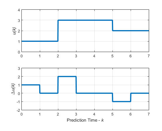
This graph corresponds to the choice moves=[2 3 2], or
equivalently, u(0)=u(1),
u(2)=u(3)=u(4),
u(5)=u(6), Δ
u(0)=z0, Δ
u(2)=z1, Δ
u(5)=z2, Δ u(1)=Δ
u(3)=Δ u(4)=Δ
u(6)=0.
Then, the corresponding matrix JM is
For more information on manipulated variable blocking, see Manipulated Variable Blocking.
Cost Function
Standard Form. The function to be optimized is
where
| (1) |
and LSy and LSu are the diagonal matrices or outputs and MV scaling factors, respectively, in engineering units.
Finally, after substituting u(k), Δu(k), y(k), J(z) can be rewritten as
| (2) |
where
Here, I1 = … = Ip are identity matrices of size nu.
Note
You might want the QP problem to remain strictly convex. If the condition number of
the Hessian matrix KΔU is larger than
1012, add the quantity 10*sqrt(eps)
on each diagonal term. You can use this solution only when all input rates are
unpenalized
(WΔu=0)
(see the Weights property of the mpc object).
Alternative Cost Function. If you are using the alternative cost function shown in Alternative Cost Function, then Equation 1 is replaced by the following:
| (3) |
In this case, the block-diagonal matrices repeat p times, for example, once for each step in the prediction horizon.
You also have the option to use a combination of the standard and alternative forms.
For more information, see the Weights property of the mpc object.
Constraints
Next, consider the limits on inputs, input increments, and outputs along with the constraint ɛ≥ 0.
Note
To reduce computational effort, the controller automatically eliminates extraneous constraints, such as infinite bounds. Thus, the constraint set used in real time might be much smaller than that suggested in this section.
Similar to what you did for the cost function, you can substitute u(k), Δu(k), y(k), and obtain
| (4) |
In this case, matrices Mz, Mɛ, Mlim, Mv, Mu, and Mx are obtained from the upper and lower bounds and ECR values.
Unconstrained Model Predictive Control
The optimal solution is computed analytically
and the model predictive controller sets Δu(k)=z*0, u(k)=u(k–1)+Δu(k).
See Also
Functions
Objects
mpc|mpcstate|mpcsimopt|mpcmoveopt