Classify Hyperspectral Images Using Deep Learning

This example shows how to classify hyperspectral images using a custom spectral convolution neural network (CSCNN) for classification.

This example requires the Hyperspectral Imaging Library for Image Processing Toolbox™. You can install the Hyperspectral Imaging Library for Image Processing Toolbox from Add-On Explorer. For more information about installing add-ons, see Get and Manage Add-Ons. The Hyperspectral Imaging Library for Image Processing Toolbox requires desktop MATLAB®, as MATLAB® Online™ and MATLAB® Mobile™ do not support the library.

Hyperspectral imaging measures the spatial and spectral features of an object at different wavelengths ranging from ultraviolet through long infrared, including the visible spectrum. Unlike color imaging, which uses only three types of sensors sensitive to the red, green, and blue portions of the visible spectrum, hyperspectral images can include dozens or hundreds of channels. Therefore, hyperspectral images can enable the differentiation of objects that appear identical in an RGB image.

This example uses a CSCNN that learns to classify 16 types of vegetation and terrain based on the unique spectral signatures of each material. The example shows how to train a CSCNN and also provides a pretrained network that you can use to perform classification.

Load Hyperspectral Data Set

This example uses the Indian Pines data set, included with the Image Processing Toolbox™ Hyperspectral Imaging Library. The data set consists of a single hyperspectral image of size 145-by-145 pixels with 220 color channels. The data set also contains a ground truth label image with 16 classes, such as Alfalfa, Corn, Grass-pasture, Grass-trees, and Stone-Steel-Towers.

Read the hyperspectral image using the hypercube function.

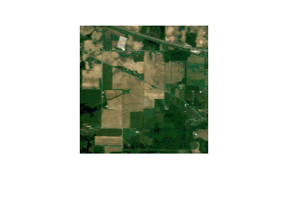
hcube = hypercube("indian_pines.dat");

Visualize a false-color version of the image using the colorize function.

rgbImg = colorize(hcube,method="rgb");
imshow(rgbImg)

Load the ground truth labels and specify the number of classes.

gtLabel = load("indian_pines_gt.mat");
gtLabel = gtLabel.indian_pines_gt;
numClasses = 16;

Preprocess Training Data

Reduce the number of spectral bands to 30 using the hyperpca function. This function performs principal component analysis (PCA) and selects the spectral bands with the most unique signatures.

dimReduction = 30;
imageData = hyperpca(hcube,dimReduction);

Normalize the image data.

sd = std(imageData,[],3);
imageData = imageData./sd;

Split the hyperspectral image into patches of size 25-by-25 pixels with 30 channels using the createImagePatchesFromHypercube helper function. This function is attached to the example as a supporting file. The function also returns a single label for each patch, which is the label of the central pixel.

windowSize = 25;
inputSize = [windowSize windowSize dimReduction];
[allPatches,allLabels] = createImagePatchesFromHypercube(imageData,gtLabel,windowSize);

indianPineDataTransposed = permute(allPatches,[2 3 4 1]);
dsAllPatches = augmentedImageDatastore(inputSize,indianPineDataTransposed,allLabels);

Not all of the cubes in this data set have labels. However, training the network requires labeled data. Select only the labeled cubes for training. Count how many labeled patches are available.

patchesLabeled = allPatches(allLabels>0,:,:,:);
patchLabels = allLabels(allLabels>0);
numCubes = size(patchesLabeled,1);

Convert the numeric labels to categorical.

patchLabels = categorical(patchLabels);

Randomly divide the patches into training and test data sets.

[trainingIdx,valIdx,testIdx] = dividerand(numCubes,0.3,0,0.7);
dataInputTrain = patchesLabeled(trainingIdx,:,:,:);
dataLabelTrain = patchLabels(trainingIdx,1);
dataInputTest = patchesLabeled(testIdx,:,:,:);
dataLabelTest = patchLabels(testIdx,1);

Transpose the input data.

dataInputTransposeTrain = permute(dataInputTrain,[2 3 4 1]); 
dataInputTransposeTest = permute(dataInputTest,[2 3 4 1]);

Create datastores that read batches of training and test data.

dsTrain = augmentedImageDatastore(inputSize,dataInputTransposeTrain,dataLabelTrain);
dsTest = augmentedImageDatastore(inputSize,dataInputTransposeTest,dataLabelTest);

Create CSCNN Classification Network

Define the CSCNN architecture.

layers = [
    image3dInputLayer(inputSize,Name="Input",Normalization="None")
    convolution3dLayer([3 3 7],8,Name="conv3d_1")
    reluLayer(Name="Relu_1")
    convolution3dLayer([3 3 5],16,Name="conv3d_2")
    reluLayer(Name="Relu_2")
    convolution3dLayer([3 3 3],32,Name="conv3d_3")
    reluLayer(Name="Relu_3")
    convolution3dLayer([3 3 1],8,Name="conv3d_4")
    reluLayer(Name="Relu_4")
    fullyConnectedLayer(256,Name="fc1")
    reluLayer(Name="Relu_5")
    dropoutLayer(0.4,Name="drop_1")
    fullyConnectedLayer(128,Name="fc2")
    dropoutLayer(0.4,Name="drop_2")
    fullyConnectedLayer(numClasses,Name="fc3")
    softmaxLayer(Name="softmax")];
net = dlnetwork(layers);

Visualize the network using Deep Network Designer.

deepNetworkDesigner(net)

Specify Training Options

Specify the required network parameters. For this example, train the network for 100 epochs with an initial learning rate of 0.001, a batch size of 256, and Adam optimization.

numEpochs = 100;
miniBatchSize = 256;
initLearningRate = 0.001;
momentum = 0.9;
learningRateFactor = 0.01;

options = trainingOptions("adam", ...
    InitialLearnRate=initLearningRate, ...
    LearnRateSchedule="piecewise", ...
    LearnRateDropPeriod=30, ...
    LearnRateDropFactor=learningRateFactor, ...
    MaxEpochs=numEpochs, ...
    MiniBatchSize=miniBatchSize, ...
    GradientThresholdMethod="l2norm", ...
    GradientThreshold=0.01, ...
    VerboseFrequency=100, ...
    ValidationData=dsTest, ...
    ValidationFrequency=100);

Train the Network

By default, the example downloads a pretrained classifier for the Indian Pines data set. The pretrained network enables you to classify the Indian Pines data set without waiting for training to complete.

To train the network, set the doTraining variable in the following code to true. Train the neural network using the trainnet (Deep Learning Toolbox) function. For classification, use cross-entropy loss. By default, the trainnet function uses a GPU if one is available. Training on a GPU requires a Parallel Computing Toolbox™ license and a supported GPU device. For information on supported devices, see GPU Computing Requirements (Parallel Computing Toolbox). Otherwise, the trainnet function uses the CPU. To specify the execution environment, use the ExecutionEnvironment training option.

doTraining = false;
if doTraining
    net = trainnet(dsTrain,net,"crossentropy",options);
    modelDateTime = string(datetime("now",Format="yyyy-MM-dd-HH-mm-ss"));
    save("trainedIndianPinesCSCNN-"+modelDateTime+".mat","net");
else
    dataDir = pwd;
    trainedNetwork_url = "https://ssd.mathworks.com/supportfiles/" + ...
        "image/data/trainedIndianPinesCSCNN_v2.mat";
    downloadTrainedNetwork(trainedNetwork_url,pwd);
    load(fullfile(dataDir,"trainedIndianPinesCSCNN_v2.mat"));
end

Classify Hyperspectral Image Using Trained CSCNN

Calculate the accuracy of the classification for the test data set. Here, accuracy is the fraction of the correct pixel classification over all the classes.

scores = minibatchpredict(net,dsTest);
predictionTest = scores2label(scores,categories(dataLabelTest));

accuracy = sum(predictionTest == dataLabelTest)/numel(dataLabelTest);
disp("Accuracy of the test data = "+accuracy)

Accuracy of the test data = 0.99805

Reconstruct the complete image by classifying all image pixels, including pixels in labeled training patches, pixels in labeled test patches, and unlabeled pixels.

predScores = minibatchpredict(net,dsAllPatches);
prediction = scores2label(predScores,categories(dataLabelTest));
prediction = double(prediction);

The network is trained on labeled patches only. Therefore, the predicted classification of unlabeled pixels is meaningless. Find the unlabeled patches and set the label to 0.

patchesUnlabeled = find(allLabels==0);
prediction(patchesUnlabeled) = 0;

Reshape the classified pixels to match the dimensions of the ground truth image.

[m,n,d] = size(imageData);
indianPinesPrediction = reshape(prediction,[n m]);
indianPinesPrediction = indianPinesPrediction';

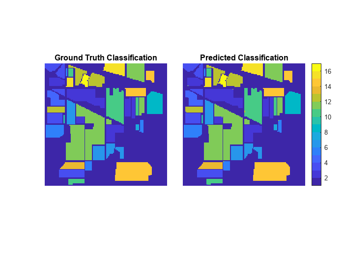
Display the ground truth and predicted classification.

cmap = parula(numClasses);

figure
tiledlayout(1,2,TileSpacing="Tight")
nexttile
imshow(gtLabel,cmap)
title("Ground Truth Classification")

nexttile
imshow(indianPinesPrediction,cmap)
colorbar
title("Predicted Classification")

To highlight misclassified pixels, display a composite image of the ground truth and predicted labels. Gray pixels indicate identical labels and colored pixels indicate different labels.

figure
imshowpair(gtLabel,indianPinesPrediction)