iopzplot

Plot pole-zero map for input-output pairs of dynamic system

Syntax

iopzplot(sys)

iopzplot(sys1,sys2,...,sysN)

iopzplot(sys1,ColorSpec1,...,sysN,ColorSpecN)

iopzplot(___,plotoptions)

iopzplot(___,Name=Value)

iopzplot(parent,___)

iopzp = iopzplot(___)

Description

The iopzplot function plots the pole-zero map for input-output pairs of a dynamic system model. To customize the plot, you can return an IOPZPlot object and modify it using dot notation. For more information, see Customize Linear Analysis Plots at Command Line (Control System Toolbox).

To obtain pole and zero locations, use the iopzmap function.

iopzplot(sys) plots the poles and zeros of each input/output pair of the dynamic system model sys. In the plot, x and o represent poles and zeros, respectively.

iopzplot(sys1,sys2,...,sysN) displays the poles and zeros of multiple models on a single plot.

iopzplot(sys1,ColorSpec1,...,sysN,ColorSpecN) sets the line style, marker type, and color for the plot of each system.

iopzplot(___,plotoptions) plots the poles and zeros with the plotting options specified in plotoptions. Settings you specify in plotoptions override the plotting preferences for the current MATLAB^® session. You can use plotoptions with any of the input argument combinations in previous syntaxes.

iopzplot(___,Name=Value) specifies response properties using one or more name-value arguments. For example, iopzplot(sys,MarkerSize=10) sets the pole and zero marker sizes to 10. (since R2026a)

When plotting responses for multiple systems, the specified name-value arguments apply to all responses.

The Color name-value argument overrides specified using the ColorSpec argument.

iopzplot(parent,___) plots the poles and zeros in the specified parent graphics container, such as a Figure or TiledChartLayout, and sets the Parent property. Use this syntax when you want to create a plot in a specified open figure or when creating apps in App Designer.

iopzp = iopzplot(___) plots the plots and zeros and returns the corresponding chart object. To customize the appearance and behavior of the response plot, modify the chart object properties using dot notation.

Examples

Change I/O Grouping on Pole/Zero Map

Create a pole/zero map of a two-input, two-output dynamic system.

sys = rss(3,2,2);
ip = iopzplot(sys);

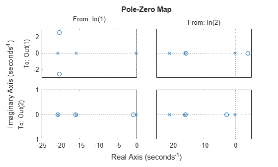
By default, the plot displays the poles and zeros of each I/O pair on its own axis. Modify the chart object to view all I/Os on a single axis.

ip.IOGrouping = "all";

Use Pole-Zero Map to Examine Identified Model

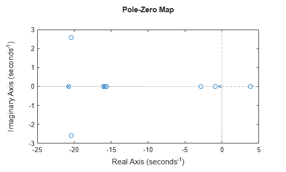
View the poles and zeros of a sixth-order state-space model estimated from input-output data. Use the plot handle to display the confidence intervals of the identified model's pole and zero locations.

load iddata1
sys = ssest(z1,6,ssestOptions('focus','simulation'));
h = iopzplot(sys);
showConfidence(h)

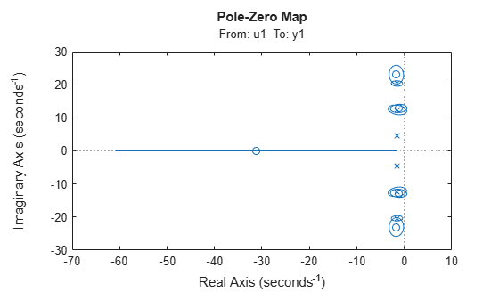
There is at least one pair of complex-conjugate poles whose locations overlap with those of a complex zero, within the 1-σ confidence region. This suggests their redundancy. Hence, a lower (4th) order model might be more robust for the given data.

sys2 = ssest(z1,4,ssestOptions('focus','simulation'));
h = iopzplot(sys,sys2);
showConfidence(h)
legend('6th-order','4th-order')
axis([-20, 10 -30 30])

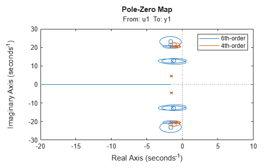
The fourth-order model sys2 shows less variability in the pole-zero locations.

Input Arguments

sys — Dynamic system

dynamic system model | model array

Dynamic system, specified as a SISO or MIMO dynamic system model or array of dynamic system models. You can use these types of dynamic systems:

• Continuous-time or discrete-time numeric LTI models, such as tf (Control System Toolbox), zpk (Control System Toolbox), or ss (Control System Toolbox) models.

• Sparse state-space models, such as sparss (Control System Toolbox) or mechss (Control System Toolbox) models.

• Generalized or uncertain LTI models such as genss (Control System Toolbox) or uss (Robust Control Toolbox) models. Using uncertain models requires Robust Control Toolbox™ software.

  • For tunable control design blocks, the function evaluates the model at its current value to plot the response.

  • For uncertain control design blocks, the function plots the nominal value and random samples of the model.

• Identified LTI models, such as idtf, idss, or idproc models.

If sys is an array of models, the plot shows responses of all models in the array on the same axes.

ColorSpec — Color

"r" | "g" | "b" | ...

Color, specified as one of the following values.

Color	Description
"r"	red
"g"	green
"b"	blue
"c"	cyan
"m"	magenta
"y"	yellow
"k"	black
"w"	white

plotoptions — Pole-zero plot options

pzoptions object

Pole-zero plot options, specified as a pzoptions object. You can use these options to customize the PZ plot appearance. Settings you specify in plotoptions override the preference settings for the current MATLAB session.

parent — Parent graphics container

Figure object | TiledChartLayout object | UIFigure object | UIGridLayout object | UIPanel object | UITab object

Parent graphics container, specified as one of these objects:

• Figure

• TiledChartLayout

• UIFigure

• UIGridLayout

• UIPanel

• UITab

Name-Value Arguments

Specify optional pairs of arguments as Name1=Value1,...,NameN=ValueN, where Name is the argument name and Value is the corresponding value. Name-value arguments must appear after other arguments, but the order of the pairs does not matter.

Example: iopzplot(sys,LegendDisplay="off") hides the response of sys from the plot legend.

Name — Response name

string | character vector

Response name, specified as a string or character vector and stored as a string.

Visible — Response visibility

"on" (default) | on/off logical value

Response visibility, specified as one of these logical on/off values:

• "on", 1, or true — Display the response in the plot.

• "off", 0, or false — Do not display the response in the plot.

The value is stored as an on/off logical value of type matlab.lang.OnOffSwitchState.

LegendDisplay — Option to list response in legend

"on" (default) | on/off logical value

Option to list the response in the legend, specified as one of these logical on/off values:

• "on", 1, or true — List the response in the legend.

• "off", 0, or false — Do not list the response in the legend.

The value is stored as an on/off logical value of type matlab.lang.OnOffSwitchState.

Color — Plot color

RGB triplet | hexadecimal color code | color name

Plot color, specified as an RGB triplet or a hexadecimal color code and stored as an RGB triplet. Specifying a color using a name-value argument overrides any color that you specify using LineSpec.

You can also specify some common colors by name. This table lists these colors and their corresponding RGB triplets and hexadecimal color codes.

Color Name	RGB Triplet	Hexadecimal Color Code
"red" or "r"	[1 0 0]	#FF0000
"green" or "g"	[0 1 0]	#00FF00
"blue" or "b"	[0 0 1]	#0000FF
"cyan" or "c"	[0 1 1]	#00FFFF
"magenta" or "m"	[1 0 1]	#FF00FF
"yellow" or "y"	[1 1 0]	#FFFF00
"black" or "k"	[0 0 0]	#000000
"white" or "w"	[1 1 1]	#FFFFFF

MarkerSize — Marker size

positive scalar

Marker size, specified as a positive scalar.

LineWidth — Line width

positive scalar

Line width, specified as a positive scalar.

SeriesIndex — Series index

positive integer | "none"

Series index, specified as a positive integer or "none".

By default, the SeriesIndex property is a number that corresponds to the order in which the response was added to the chart, starting at 1. MATLAB uses the number to calculate indices for automatically assigning color, line style, or markers for responses. Any responses in the chart that have the same SeriesIndex number also have the same color, line style, and markers.

A SeriesIndex value of "none" indicates that a response does not participate in the indexing scheme.

Output Arguments

iopzp — Chart object

IOPZPlot object

Chart object, returned as a IOPZPlot object. To customize your plot appearance and behavior, modify the properties of this object using dot notation. For more information, see IOPZPlot Properties (Control System Toolbox).

More About

Pole-Zero Plot Grid Lines

To plot lines of constant damping ratio (ζ) and natural frequency (w_n in the s-plane or z-plane, enable the GridVisible property of the chart object. Alternatively, you can use the grid command or right-click the plot area and select Grid.

The type of grid displayed in the plot depends on the time-domain of the plotted responses.

• For z-plane grids, you can specify the grid sample time (T_s) using the GridSampleTime property of the chart object. The w_n grid lines depend on the T_s. Therefore, you must specify T_s to plot specific w_n values. If you do not specify T_s, the plot uses normalized factors of w_n/T_s.

• The default s-plane grid plots lines for ζ from 0 to 1 in steps of 0.1 and w_n from 0 to 10 rad/sec in steps of one rad/sec.

• The default z-plane grid plots lines for ζ from 0 to 1 in steps of 0.1 and w_n from 0 to π/T_s in steps of 0.1*π/T_s.

• To specify ζ and w_n values, set the GridDampingSpec and GridFrequencySpec properties of the chart object.

Tips

• Plots created using iopzplot do not support multiline titles or labels specified as string arrays or cell arrays of character vectors. To specify multiline titles and labels, use a single string with a newline character.

  iopzplot(sys)
  title("first line" + newline + "second line");

Version History

Introduced in R2012a

R2026a: Specify response properties using name-value arguments

You can now specify response properties using name-value arguments.

When plotting responses for multiple systems, the specified property values apply to all responses.

If a name-value argument sets the same property as another input argument, the property value is set to the name-value argument.

R2026a: Specifying axes object as parent not recommended

Specifying an Axes object or a UIAxes object as the parent container of a linear analysis plot is not recommended. Instead, specify the parent container as one of these objects:

• Figure

• TiledChartLayout

• UIFigure

• UIGridLayout

• UIPanel

• UITab

R2025a: Add grid lines for constant damping factors and natural frequencies for MIMO systems

You can now add grid lines for constant damping factors and natural frequencies to MIMO iopzplot charts using sgrid (Control System Toolbox) and zgrid (Control System Toolbox).

R2024b: Improved customization workflows and integration with MATLAB plotting tools

Starting in R2024b, the iopzplot function returns an IOPZPlot chart object. Previously, the iopzplot function returned a handle to the resulting plot.

The new chart object allows you to customize your plot using dot notation.

The new chart object also improves integration with MATLAB plotting tools. For example:

• You can now add PZ plots to tiled chart layouts.

• Saving and loading a parent figure now maintains full plot interactivity.

• You can add a response to your PZ plot using the new addResponse function.

The following functionality changes might require updates to your code:

• The gca function now returns the chart object rather than an axes within the plot.

• You can no longer access the graphics objects within a PZ plot using the Children property of its parent figure.