Estimate State-Space Model

Estimate state-space model using time or frequency data in the Live Editor

Since R2019b

Description

The Estimate State-Space Model task lets you interactively estimate and validate a state-space model using time or frequency data. You can define and vary the model structure and specify optional parameters, such as initial condition handling and search method. The task automatically generates MATLAB^® code for your live script. For more information about Live Editor tasks generally, see Add Interactive Tasks to a Live Script.

State-space models are models that use state variables to describe a system by a set of first-order differential or difference equations, rather than by one or more nth-order differential or difference equations. State variables can be reconstructed from the measured input-output data, but are not themselves measured during the experiment.

The state-space model structure is a good choice for quick estimation because it requires you to specify only one input, the model order. For more information about state-space estimation, see What Are State-Space Models?

The Estimate State-Space Model task is independent of the more general System Identification app. Use the System Identification app when you want to compute and compare estimates for multiple model structures.

To get started, load experiment data that contains input and output data into your MATLAB workspace and then import that data into the task. Then specify a model structure to estimate. The task gives you controls and plots that help you experiment with different model parameters and compare how well the output of each model fits the measurements.

More

Related Functions

The code that Estimate State-Space Model generates uses the following functions.

• iddata

• idfrd

  frd (Control System Toolbox)

• ssest

• ssestOptions

• compare

The task estimates an idss state-space model.

×

Open the Task

To add the Estimate State-Space Model task to a live script in the MATLAB Editor:

• On the Live Editor tab, select Task > Estimate State-Space Model.

• In a code block in your script, type a relevant keyword, such as state, space, or estimate. Select Estimate State Space Model from the suggested command completions.

Examples

Estimate State-Space Model with Live Editor Task

Use the Estimate State-Space Model Live Editor Task to estimate a state-space model and compare the model output to the measurement data.

Open this example to see a preconfigured script containing the task.

Set Up Data

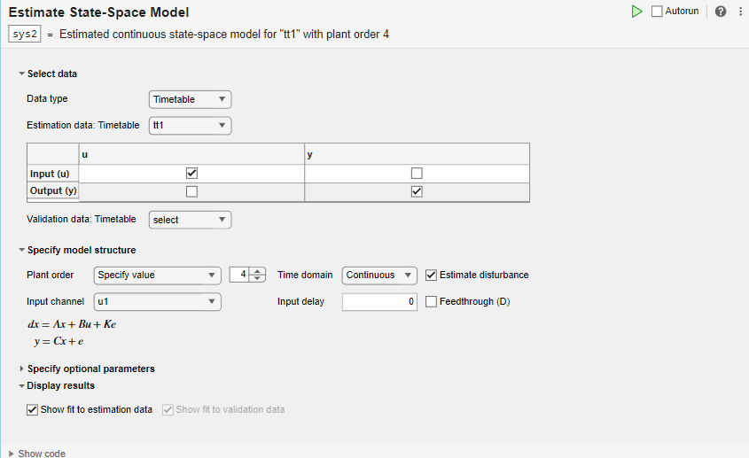
Load the measurement data iddata1 into your MATLAB workspace.

load iddata1 z1
z1

z1 =

Time domain data set with 300 samples.
Sample time: 0.1 seconds               
                                       
Outputs      Unit (if specified)       
   y1                                  
                                       
Inputs       Unit (if specified)       
   u1                                  
                                       

Import Data into the Task

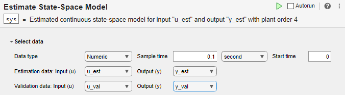
In the Select data section, set Data Type to Data Object and set Estimation Object to z1.

The data object contains the input and output variable names as well as the sample time, so you do not have to specify them.

Estimate the Model Using Default Settings

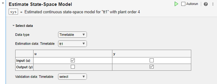
Examine the model structure and optional parameters.

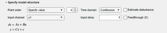
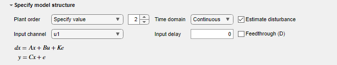
In the Specify model structure section, the plant order is set to its default value of 4 and the model is in the continuous-time domain. Equations below the parameters in this section display the specified structure.

In the Specify optional parameters section, parameters display the default options for state-space estimation.

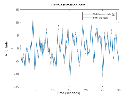
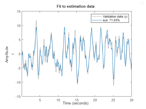
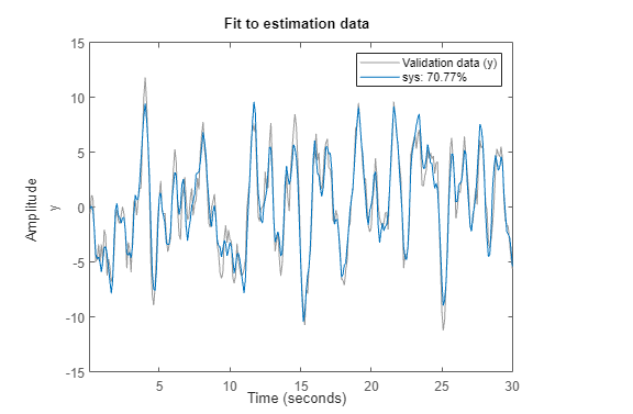
Execute the task from the Live Editor tab using Run. A plot displays the estimation data, the estimated model output, and the fit percentage.

Experiment with Parameter Settings

Experiment with the parameter settings and see how they influence the fit.

For instance, in Specify model structure, the Estimate disturbance box is selected, so the disturbance matrix K is present in the equations. If you clear the box, the K term disappears. Run the updated configuration, and see how the fit changes.

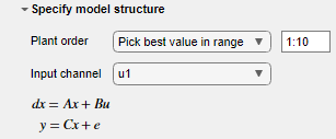
Change the Plant Order setting to Pick best value in range. The default setting is 1:10.

When you run the model, a Model Order Selection plot displays the contribution of each state to the model dynamic behavior. With the initial task settings for the other parameters, the plot displays a recommendation of 2 for the model order.

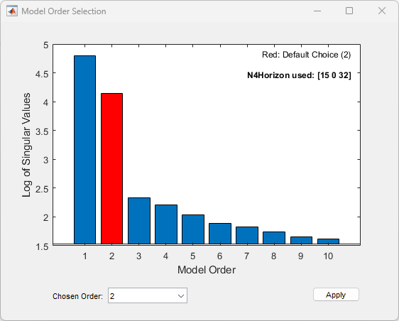
Accept this recommendation by clicking Apply, and see how this change affects the fit.

Generate Code

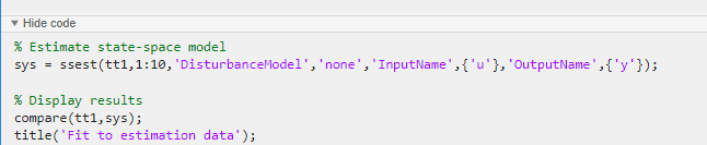
To display the code that the task generates, click at the bottom of the parameter section. The code that you see reflects the current parameter configuration of the task.

Use Validation Data Set to Validate Estimated Model

Use separate estimation and validation data so that you can validate the estimated state-space model.

Open this example to see a preconfigured script containing the task.

Set Up Data

Load measurement data iddata1 into your MATLAB workspace and examine its contents.

load iddata1 z1
z1

z1 =

Time domain data set with 300 samples.
Sample time: 0.1 seconds               
                                       
Outputs      Unit (if specified)       
   y1                                  
                                       
Inputs       Unit (if specified)       
   u1                                  
                                       

Extract the input and output measurements.

u = z1.u;
y = z1.y;

Split the data into two sets, with one half for estimation and one half for validation. The original data set has 300 samples, so each new data set has 150 samples.

u_est = u(1:150);
u_val = u(151:300);
y_est = y(1:150);
y_val = y(151:300);

Import Data into Task

In the Select data section, set Data Type to Time. Set Sample Time to 0.1 seconds, which is the sample time in the original iddata object z1. Select the appropriate data sets for estimation and validation.

Estimate and Validate Model

The example Estimate State-Space Model with Live Editor Task recommends a model order of 2. Use that value for Plant Order. Leave other parameters at their default values. Note that Input Channel refers not to the input data set, but to the channel index within the input data set, which for a single-input system is always u1.

Execute the task from the Live Editor tab using Run. Executing the task creates two plots. The first plot shows the estimation results and the second plot shows the validation results.

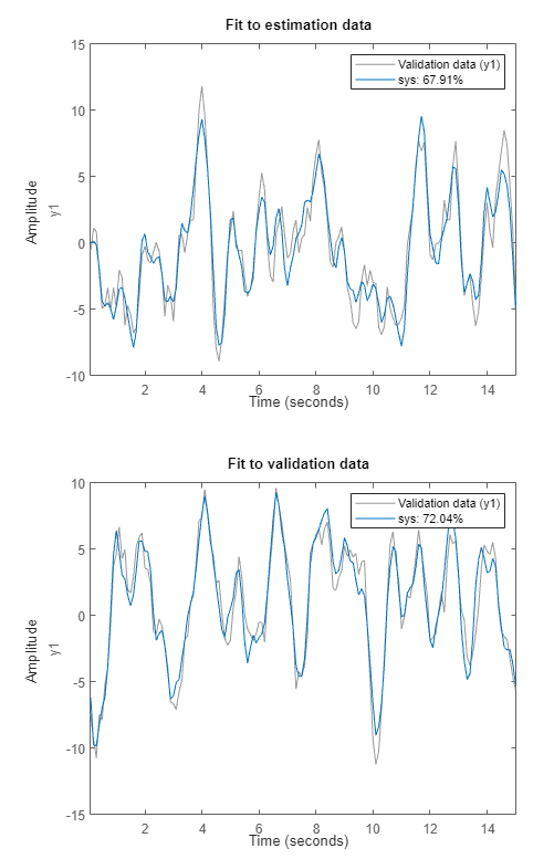
The fit to the estimation data is somewhat worse than in Estimate State-Space Model with Live Editor Task. Estimation in the current example has only half the data with which to estimate the model. The fit to the validation data, which represents the goodness of the model more generally, is better than the fit to the estimation data.

Parameters

Select Data

Data Type — Data type for input and output data

Time (default) | Frequency | Data Object

The task accepts numeric measurement values that are uniformly sampled in time. Input and output signals can contain multiple channels. Data can be packaged as numeric arrays (for Time or Frequency) or in a data object, such as an iddata or idfrd object.

The data type you choose determines whether you must specify additional parameters.

• Time — Specify Sample Time and Start Time in the time units that you select.

• Frequency — Specify Frequency by selecting the variable name of a frequency vector in your MATLAB workspace. Specify the units for this frequency vector. Specify Sample Time in seconds.

• Data Object — Specify no additional parameters because the data object already contains information on time or frequency sampling.

Estimation Input (u) and Estimation Output (y) — Variable names of input and output data for estimation

valid variable names

Select the input and output variable names from the MATLAB workspace choices. Use these parameters when Data Type is Time or Frequency.

Estimation Object — Variable name of data object containing input and output data for estimation

valid variable name

Select the data object variable name from the MATLAB workspace choices. Use this parameter when Data Type is Data Object.

Validation Input (u) and Validation Output (y) — Variable names of input and output data for validation

valid variable names

Select the input and output variable names from the workspace choices. Use these parameters when Data Type is Time or Frequency. Specifying validation data is optional but recommended.

Validation Object — Variable name of data object containing input and output data for validation

valid variable name

Select the data object variable name from the MATLAB workspace choices. Use this parameter when Data Type is Data Object. Specifying validation data is optional but recommended.

Specify Model Structure

Plant Order — Order of model to estimate

4 (default) | integer scalar | integer range

The task allows you to specify a single value or a range of values for the order of the model to estimate.

• Specify value — Specify the order of the model explicitly.

• Pick best value in range — Specify a range of values, such as 1:10. When you run the task, the Hankel singular-value plot visualizes the relative energy contribution of each state in the estimated model and recommends the lowest order that reproduces critical dynamic behavior. Proceed with this recommendation or select another order in Chosen Order. Click Apply to accept the model order and proceed.

Time Domain — Continuous or discrete time domain

Continuous (default) | Discrete

Select a continuous-time or discrete-time model.

Estimate Disturbance — Include disturbance in estimation model

off (default) | on

Select this option to estimate the disturbance model. When you select this option, the model equations update to show the K matrix and e term.

Input Channel — Set input channel delay and feedthrough options

u1 (default) | u2 | ...

For each input channel, assign values for Input Delay and Feedthrough.

• Input Channel — Select an input channel. The input channel is always of the form ui, where i is the ith channel of the input u.

• Input Delay — Enter the input delay in number of samples (discrete-time model) or number of time units (continuous-time model) for the channel. For instance, to specify a 0.2-second input delay for a continuous-time system for which the time unit is milliseconds, enter 200.

• Feedthrough — Select this option to estimate channel feedthrough from input to output. When you select this option, the model equations update to show the Du term.

Specify Optional Parameters

Fit Focus — Minimize prediction error or simulation error

Prediction (default) | Simulation

Fit focus specifies what error to minimize in the loss function during estimation.

• Prediction — Minimize the one-step-ahead prediction error between measured and predicted outputs. This estimation approach focuses on producing a good predictor model for the estimation inputs and outputs. Prediction focus generally produces the best estimation results because it uses both input and output measurements, thus accounting for disturbances.

• Simulation — Minimize the error between measured and simulated outputs. This estimation approach focuses on producing a simulated model response that has a good fit with the estimation inputs and outputs. Simulation focus is generally best for validation, especially with data sets not used for the original estimation.

Initial Conditions — Handling of initial states

Auto (default) | Zero | Estimate | Backcast

Set this option when you want to choose a specific method for initializing the model states. With the default setting of Auto, the software chooses the method based on the estimation data. Choices are:

• Zero — The initial state is set to zero.

• Estimate — The initial state is treated as an independent estimation parameter.

• Backcast — The initial state is estimated using the best least-squares fit.

Input Intersampling — Intersampling behavior for input signal

Zero-order hold (default) | Triangle approximation | Band-limited

Input intersampling is a property of the input data. The task uses this property when estimating continuous models. Specify Input Intersampling when your data type is Time or Frequency. If you are using an iddata object, the object already contains the intersampling information. Choices for this property are:

• Zero-order hold — Piecewise-constant input signal between samples

• Triangle approximation — Piecewise-linear input signal between samples, also known as first-order hold

• Band-limited — Input signal has zero power above the Nyquist frequency

Search Method — Numerical search mode for iterative parameter estimation

Auto (default) | Gauss-Newton | Adaptive Gauss-Newton | Levenberg-Marquardt | Gradient Search

• Auto — For each iteration, the software cycles through the methods until it finds the first direction descent that leads to a reduction in estimation cost.

• Gauss-Newton — Subspace Gauss-Newton least-squares search.

• Levenberg-Marquardt — Levenberg-Marquardt least-squares search.

• Adaptive Gauss-Newton —Adaptive subspace Gauss-Newton search.

• Gradient Search — Steepest descent least-squares search.

Max. Iterations — Maximum number of iterations during error minimization

20 (default) | positive integer

Set the maximum number of iterations during error minimization. The iterations stop when Max. Iterations is reached or another stopping criterion is satisfied, such as Tolerance.

Tolerance — Minimum percentage of expected improvement in error

0.01 (default) | positive integer

When the percentage of expected improvement is less than Tolerance, the iterations stop.

Weighting Prefilter — Weighting prefilter for loss function

No filter (default) | Passband(s) | LTI Filter | Frequency weights vector | Inverse of magnitude of the frequency response | Inverse of square root of magnitude of the frequency response

Set this option when you want to apply a weighting prefilter to the loss function that the task minimizes when you estimate the model. When you select an option, you must also select the associated variable in your workspace that contains the filter information. The available options depend on the domain of the data.

Weighting Prefilter	Data Domain	Filter Information
No Filter	Time and frequency
Passbands	Time and frequency	Passband ranges, specified as a 1-by-2 row vector or an n-by-2 matrix, where n is the number of passbands.
LTI Filter	Time and frequency	SISO LTI model.
Frequency Weights Vector	Frequency	Frequency weights, specified as a column vector with the same length as the frequency vector.
Inverse of magnitude of the frequency response	Frequency response	The weighting filter is$$1/|G(\omega )|$$, where G(ω) is the complex frequency-response data. SISO and SIMO systems only.
Inverse of square root of magnitude of the frequency response	Frequency response	The weighting filter is $$1/\sqrt{|G(\omega )|}$$. SISO and SIMO systems only.

For instance, suppose that you are performing estimation with SISO frequency-domain data and that in your MATLAB workspace, you have a column vector W that contains frequency weights for the prefilter. In the task, select Weighting prefilter > Frequency weights vector and the variable W.

Visualize Results

Output Plot — Plot comparison of model and measured outputs

on (default) | off

Plot a comparison of the model output and the original measured data, along with the fit percentage. If you have separate validation data, a second plot compares the model response to the validation input data with the measured output from the validation data set.

Version History

Introduced in R2019b