Troubleshooting Multivariate Normal Regression
This section provides a few pointers to handle various technical and operational difficulties that might occur.
Biased Estimates
If samples are ignored, the number of samples used in the estimation
is less than NumSamples. Clearly the actual number
of samples used must be sufficient to obtain estimates. In addition,
although the model parameters Parameters (or mean
estimates Mean) are unbiased maximum likelihood
estimates, the residual covariance estimate Covariance is
biased. To convert to an unbiased covariance estimate, multiply Covariance by
where Count is the actual number of samples
used in the estimation with Count ≤ NumSamples. None of the regression
functions perform this adjustment.
Requirements
The regression functions, particularly the estimation functions,
have several requirements. First, they must have consistent values
for NumSamples, NumSeries, and NumParams.
As a rule, the multivariate normal regression functions require
and the least-squares regression functions require
where Count is the actual number of samples
used in the estimation with
Second, they must have enough nonmissing values to converge. Third, they must have a nondegenerate covariance matrix.
Although some necessary and sufficient conditions can be found in the references, general conditions for existence and uniqueness of solutions in the missing-data case, do not exist. Nonconvergence is usually due to an ill-conditioned covariance matrix estimate, which is discussed in greater detail in Nonconvergence.
Slow Convergence
Since worst-case convergence of the ECM algorithm is linear, it is possible to execute
hundreds and even thousands of iterations before termination of the algorithm. If
you are estimating with the ECM algorithm regularly with regular updates, you can
use prior estimates as initial guesses for the next period's estimation. This
approach often speeds up things since the default initialization in the regression
functions sets the initial parameters b to zero and the initial
covariance C to be the identity matrix.
Other improvised approaches are possible although most approaches are problem-dependent. In
particular, for mean and covariance estimation, the estimation function ecmnmle uses a function ecmninit to obtain an initial
estimate.
Nonrandom Residuals
Simultaneous estimates for parameters b and covariances
C require C to be positive-definite. So,
the general multivariate normal regression routines require nondegenerate residual
errors. If you are faced with a model that has exact results, the least-squares
routine ecmlsrmle still works, although it
provides a least-squares estimate with a singular residual covariance matrix. The
other regression functions fail.
Nonconvergence
Although the regression functions are robust and work for most
“typical” cases, they can fail to converge. The main
failure mode is an ill-conditioned covariance matrix, where failures
are either soft or hard. A soft failure wanders endlessly toward a
nearly singular covariance matrix and can be spotted if the algorithm
fails to converge after about 100 iterations. If MaxIterations is
increased to 500 and display mode is initiated (with no output arguments),
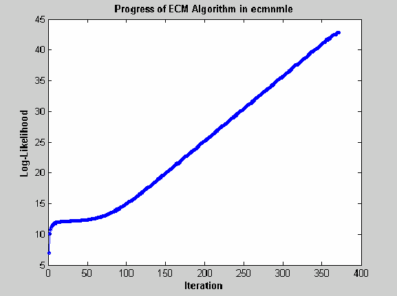
a typical soft failure looks like this.

This case, which is based on 20 observations of five assets
with 30% of data missing, shows that the log-likelihood goes linearly
to infinity as the likelihood function goes to 0. In this case, the
function converges but the covariance matrix is effectively singular
with a smallest eigenvalue on the order of machine precision (eps).
For the function ecmnmle, a hard error looks like
this:
> In ecmninit at 60
  In ecmnmle at 140
??? Error using ==> ecmnmle
Full covariance not positive-definite in iteration 218.
From a practical standpoint, if in doubt, test your residual
covariance matrix from the regression routines to ensure that it is
positive-definite. This is important because a soft error has a matrix
that appears to be positive-definite but actually has a near-zero-valued
eigenvalue to within machine precision. To do this with a covariance
estimate Covariance, use cond(Covariance),
where any value greater than 1/eps should be considered
suspect.
If either type of failure occurs, however, note that the regression routine is indicating that something is probably wrong with the data. (Even with no missing data, two time series that are proportional to one another produce a singular covariance matrix.)
See Also
mvnrmle | mvnrstd | mvnrfish | mvnrobj | ecmmvnrmle | ecmmvnrstd | ecmmvnrfish | ecmmvnrobj | ecmlsrmle | ecmlsrobj | ecmmvnrstd | ecmmvnrfish | ecmnmle | ecmnstd | ecmnfish | ecmnhess | ecmnobj | convert2sur | ecmninit