Main Content

irfplot

Plot impulse response function (IRF) of state-space model

Since R2020b

Description

irfplot plots the IRFs of the state and measurement variables in a state-space model. To return the IRFs as numeric arrays instead, use irf. Other state-space model tools to characterize the dynamics of a specified system include:

  • The forecast error variance decomposition (FEVD), computed by fevd, provides information about the relative importance of each state disturbance in affecting the forecast error variance of all measurement variables in the system.

  • Model-implied temporal correlations, computed by corr for a standard state-space model, measure the association between present and past state or measurement variables, as prescribed by the form of the model.

Fully Specified State-Space Model

example

irfplot(Mdl) plots the IRF, or dynamic response, of each state and measurement variable of the fully specified state-space model Mdl, such as an estimated model. irfplot plots a figure containing the IRFs of the measurement variables yt, and plots a separate figure containing the IRFs of the state variables xt. Each figure contains a subplot for each variable and state disturbance combination; subplot (i,j) is the IRF of variable j resulting from a unit shock applied to a state disturbance i ui,t. Subplot titles identify the shocked variable and IRF variable.

example

irfplot(Mdl,Name,Value) uses additional options specified by one or more name-value pair arguments. For example, 'PlotU',1:2,'PlotX',[] plots only the measurement variable IRFs resulting from shocks applied to the first and second state-disturbance variables (the state variable IRF plot is suppressed).

Partially Specified State-Space Model and Confidence Interval Estimation

example

irfplot(___,'Params',estParams) plots the IRFs of the partially specified state-space model Mdl using any of the input argument combinations in the previous syntaxes. estParams specifies estimates of all unknown parameters in the model.

example

irfplot(___,'Params',estParams,'EstParamCov',EstParamCov) also plots pointwise lower and upper 95% Monte Carlo confidence bounds in each plot. EstParamCov specifies the estimated covariance matrix of the parameter estimates, as returned by the estimate function, and is required for confidence interval estimation.

Customize Figures

example

irfplot(ax,___) plots on the axes objects specified by ax instead of new figures. The option ax can precede any of the input argument combinations in the previous syntaxes.

example

h = irfplot(ax,___) also returns an array of plot handles h. Use h to modify properties of the plots after you create them.

Examples

collapse all

Explicitly create the state-space model

xt=0.5xt-1+0.2utyt=2xt+0.01εt.

A = 0.5;
B = 0.2;
C = 2;
D = 0.01;
Mdl = ssm(A,B,C,D)
Mdl = 
State-space model type: ssm

State vector length: 1
Observation vector length: 1
State disturbance vector length: 1
Observation innovation vector length: 1
Sample size supported by model: Unlimited

State variables: x1, x2,...
State disturbances: u1, u2,...
Observation series: y1, y2,...
Observation innovations: e1, e2,...

State equation:
x1(t) = (0.50)x1(t-1) + (0.20)u1(t)

Observation equation:
y1(t) = (2)x1(t) + (0.01)e1(t)

Initial state distribution:

Initial state means
 x1 
  0 

Initial state covariance matrix
     x1   
 x1  0.05 

State types
     x1     
 Stationary 

Mdl is an ssm model object. Because all parameters have known values, the object is fully specified.

Plot the IRFs of the measurement and state variables.

irfplot(Mdl);

The plot entitled U1 -> Y1 is the IRF of yt, and the plot entitled U1 -> X1 is the IRF of xt. Both IRFs indicate that the effects of the shock on the system diminish after about 8 periods.

Plot the measurement variable IRF and the 95% confidence intervals on the true IRFs.

Assume that the data generating process (DGP) is the AR(1) model

xt=1+0.75xt-2+ut,

where ut is a series of independent and identically distributed Gaussian variables with mean 0 and variance 1.

Simulate 500 observations from the model.

rng(1); % For reproducibility
DGP = arima('Constant',1,'AR',{0 0.75},'Variance',1);
y = simulate(DGP,500);

Explicitly create a diffuse state-space model template for estimation that represents the model. Fit the model to the data, and return parameter estimates and their corresponding estimated covariance matrix.

A = [0 NaN NaN; 0 1 0; 1 0 0];
B = [NaN; 0; 0];
C = [1 0 0];
D = 0;
Mdl = dssm(A,B,C,D,'StateType',[0 1 0]);
[~,estParams,EstParamCov] = estimate(Mdl,y,abs(randn(3,1)));
Method: Maximum likelihood (fminunc)
Effective Sample size:            500
Logarithmic  likelihood:     -892.214
Akaike   info criterion:      1790.43
Bayesian info criterion:      1803.07
      |     Coeff      Std Err   t Stat     Prob  
--------------------------------------------------
 c(1) | 0.41320       0.12199    3.38730  0.00071 
 c(2) | 0.67319       0.02749   24.48749   0      
 c(3) | 1.11450       0.03623   30.76557   0      
      |                                           
      |  Final State   Std Dev    t Stat    Prob  
 x(1) | 3.69929        0          Inf      0      
 x(2) |  1             0          Inf      0      
 x(3) | 1.43378        0          Inf      0      

Mdl is a fully specified, estimated dssm model object.

Plot the IRF, with its 95% confidence intervals, of the measurement variable.

irfplot(Mdl,'Params',estParams,'EstParamCov',EstParamCov,...
    'PlotX',[]);

The blue line represents the estimated IRF of yt. The dashed red lines represent the upper and lower, pointwise 95% confidence bounds on the true IRF. The model has only one lag term (lag 2), as the shock filters through the system, it impacts the first state variable during odd periods only.

Simulate data from a known model, fit the data to a state-space model, and then the plot cumulative IRFs, with corresponding confidence bounds, of the estimated model to specified axes.

Assume that the data generating process (DGP) is the AR(1) model

xt=1+0.75xt-2+ut,

where ut is a series of independent and identically distributed Gaussian variables with mean 0 and variance 1.

Simulate 500 observations from the model.

rng(1); % For reproducibility
DGP = arima('Constant',1,'AR',{0 0.75},'Variance',1);
y = simulate(DGP,500);

Explicitly create a state-space model template for estimation that represents the model

xt=c+ϕxt-2+ηutyt=xt.

A = [0 NaN NaN; 0 1 0; 1 0 0];
B = [NaN; 0; 0];
C = [1 0 0];
D = 0;
Mdl = ssm(A,B,C,D,'StateType',[0 1 0]);

Fit the model template to the data. Specify a set of positive, random standard Gaussian starting values for the three model parameters. Return the estimated model, the vector of estimated parameters, and the estimated parameter covariance matrix.

[EstMdl,estParams,EstParamCov] = estimate(Mdl,y,abs(randn(3,1)));
Method: Maximum likelihood (fminunc)
Sample size: 500
Logarithmic  likelihood:     -892.214
Akaike   info criterion:      1790.43
Bayesian info criterion:      1803.07
      |     Coeff      Std Err   t Stat     Prob  
--------------------------------------------------
 c(1) | 0.41320       0.12199    3.38730  0.00071 
 c(2) | 0.67319       0.02749   24.48749   0      
 c(3) | 1.11450       0.03623   30.76557   0      
      |                                           
      |  Final State   Std Dev    t Stat    Prob  
 x(1) | 3.69929        0          Inf      0      
 x(2) |  1             0          Inf      0      
 x(3) | 1.43378        0          Inf      0      

EstMdl is a fully specified dssm model object.

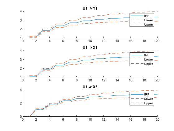
Plot the cumulative IRFs, with corresponding confidence bounds, of the first and third state variables, and the measurement variable, of the estimated model by supplying the model template Mdl, the vector of estimated parameters estParams, and the estimated parameter covariance matrix EstParamCov. Return the plot in the same figure, on three separate subplots.

ax = gobjects(3,1);
for j = 1:numel(ax)
    ax(j) = subplot(3,1,j);
end
irfplot(ax,Mdl,'Params',estParams,'EstParamCov',EstParamCov, ...
    'Cumulative',true,'PlotX',[1 3]);

Because yt=xt, the top two IRFs in the figure are equivalent. Because x1,t-1=x3,t, the IRF in the subplot at the bottom of the figure is shifted to the left, relative to the other two plots.

Plot the 10-period IRFs of only the measurement variables in a system.

Explicitly create the multivariate diffuse state-space model

x1,t=x1,t-1+0.2u1,tx2,t=x1,t-1+0.3x2,t-1+u2,ty1,t=x1,t+ε1,ty2,t=x1,t+x2,t+ε2,t.

A = [1 0; 1 0.3];
B = [0.2 0; 0 1];
C = [1 0; 1 1];
D = eye(2);
Mdl = dssm(A,B,C,D)
Mdl = 
State-space model type: dssm

State vector length: 2
Observation vector length: 2
State disturbance vector length: 2
Observation innovation vector length: 2
Sample size supported by model: Unlimited

State variables: x1, x2,...
State disturbances: u1, u2,...
Observation series: y1, y2,...
Observation innovations: e1, e2,...

State equations:
x1(t) = x1(t-1) + (0.20)u1(t)
x2(t) = x1(t-1) + (0.30)x2(t-1) + u2(t)

Observation equations:
y1(t) = x1(t) + e1(t)
y2(t) = x1(t) + x2(t) + e2(t)

Initial state distribution:

Initial state means
 x1  x2 
  0   0 

Initial state covariance matrix
     x1   x2  
 x1  Inf  0   
 x2  0    Inf 

State types
    x1       x2   
 Diffuse  Diffuse 

Mdl is a fully specified ssm model object.

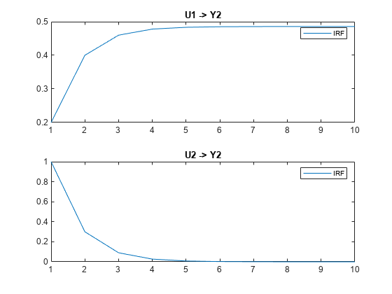
Plot the two 10-period IRFs of y2,t, and suppress the state variable IRFs.

irfplot(Mdl,'NumPeriods',10,'PlotY',2,'PlotX',[]);

The top subplot is the IRF of y2,t resulting from a shock to u1,t, which is persistent because the shock filters through the random walk state x1,t.

The bottom subplot is the IRF of y2,t resulting from a shock to u2,t, which is transient and eventually diminishes as time elapses because the state x2,t exhibits autoregressive behavior.

Simulate data from a time-varying state-space model, fit a model to the data, then plot the time-varying IRF of the estimated model.

Consider the DGP represented by this system

xt={0.75xt-1+ut;t<11-0.1xt-1+3ut;t11yt=1.5xt+2εt.

Write a function that specifies how the parameters params map to the state-space model matrices. Save this code as a file named timeVariantAR1ParamMap.m on your MATLAB® path. Alternatively, open the example to access the function.

type timeVariantAR1ParamMap.m
% Copyright 2020 The MathWorks, Inc.

function [A,B,C,D] = timeVariantAR1ParamMap(params)
% Time-varying state-space model parameter mapping function example. This
% function maps the vector params to the state-space matrices (A, B, C, and
% D). From periods 1 through 10, the state model is an AR(1)model, and from
% periods 11 through 20, the state model is possibly a different AR(1)
% model. The measurement equation is the same throughout the time span.
    A1 = {params(1)};
    A2 = {params(2)};
    varu1 = exp(params(3));  % Positive variance constraints
    varu2 = exp(params(4));
    B1 = {sqrt(varu1)}; 
    B2 = {sqrt(varu2)};
    C = params(5);
    vare1 = exp(params(6));
    D = sqrt(vare1);
    A = [repmat(A1,10,1); repmat(A2,10,1)];
    B = [repmat(B1,10,1); repmat(B2,10,1)];
end

Implicitly create a partially specified state-space model representing the DGP. For this example, fix the measurement-sensitivity coefficient C to 1.5.

C = 1.5;
fixCParamMap = @(x)timeVariantAR1ParamMap([x(1:4), C, x(5)]);
DGP = ssm(fixCParamMap);

Simulate 20 observations from the DGP. Because DGP is partially specified, pass the true parameter values to simulate by using the 'Params' name-value pair argument.

rng(10) % For reproducibility
A1 = 0.75;
A2 = -0.1; 
B1 = 1;
B2 = 3;
D = 2;
trueParams = [A1 A2 2*log(B1) 2*log(B2) 2*log(D)]; % Transform variances for parameter map
y = simulate(DGP,20,'Params',trueParams);

y is a 20-by-1 vector of simulated measurements yt from the DGP.

Because DGP is a partially specified, implicit model object, its parameters are unknown. Therefore, it can serve as a model template for estimation.

Fit the model to the simulated data. Specify random standard Gaussian draws for the initial parameter values. Return the parameter estimates.

[~,estParams] = estimate(DGP,y,randn(1,5),'Display','off')
estParams = 1×5

    0.6164   -0.1665    0.0135    1.6803   -1.5855

estParams is a 1-by-5 vector of parameter estimates. The output argument list of the parameter mapping function determines the order of the estimates: A{1}, A{2}, B{1}, B{2}, and D.

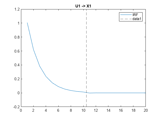
Plot the IRF of the measurement and state variables by supplying DGP (not the estimated model) and the estimated parameters by using the 'Params' name-value pair argument.

h = irfplot(DGP,'Params',estParams);
xline(h(1,1).Parent,10.5,'--')

xline(h(1,2).Parent,10.5,'--')

The figures show time-varying IRFs of the measurement and state variables. The first 10 periods correspond to the IRF of the first state equation. During period 11, what remains of the shock transfers to the second state equation, and filters through that system until it diminishes.

Input Arguments

collapse all

State-space model, specified as an ssm model object returned by ssm or its estimate function, or a dssm model object returned by dssm or its estimate function.

If Mdl is partially specified (that is, it contains unknown parameters), specify estimates of the unknown parameters by using the 'Params' name-value argument. Otherwise, irfplot issues an error.

irfplot issues an error when Mdl is a dimension-varying model, which is a time-varying model containing at least one variable that changes dimension during the sampling period (for example, a state variable drops out of the model).

Tip

If Mdl is fully specified, you cannot estimate confidence bounds. To estimate confidence bounds:

  1. Create a partially specified state-space model template for estimation Mdl.

  2. Estimate the model by using the estimate function and data. Return the estimated parameters estParams and estimated parameter covariance matrix EstParamCov.

  3. Pass the model template for estimation Mdl to irfplot, and specify the parameter estimates and covariance matrix by using the 'Params' and 'EstParamCov' name-value arguments.

  4. For the irfplot function, return the appropriate output arguments for lower and upper confidence bounds.

Axes on which to plot the IRFs, specified as a pU*(pY + pX)-by-1 vector of Axes objects, where pU, pY, and pX are the lengths of the values of the 'PlotU', 'PlotY', and 'PlotX' name-value pair arguments, respectively.

irfplot plots IRFs to the axes in ax in this order.

  1. IRFs of all measurement variables PlotY(:) resulting from a shock to the first state disturbance PlotU(1).

  2. IRFs of all measurement variables PlotY(:) resulting from a shock to the second state disturbance PlotU(2).

  3. Continue the procedure similarly until irfplot plots the IRF associated with the last state disturbance PlotU(end).

  4. Repeat steps 1 through 3, but replace the measurement variables with the state variables PlotX.

By default, irfplot plots the measurement-variable IRFs to the axes of subplots in a new figure, and plots the state-variable IRFs to the axes of subplots in another new figure.

Name-Value Arguments

Specify optional pairs of arguments as Name1=Value1,...,NameN=ValueN, where Name is the argument name and Value is the corresponding value. Name-value arguments must appear after other arguments, but the order of the pairs does not matter.

Before R2021a, use commas to separate each name and value, and enclose Name in quotes.

Example: 'PlotU',1:2,'PlotX',[] plots only the measurement-variable IRFs resulting from shocks applied to the first and second state-disturbance variables (the state-variable IRF plot is suppressed).

IRF Options

collapse all

Number of periods for which irfplot computes the IRF, specified as a positive integer. Periods in the IRF start at time 1 and end at time NumPeriods.

Example: 'NumPeriods',10 specifies the inclusion of 10 consecutive time points in the IRF starting at time 1, during which irfplot applies the shock, and ending at time 10.

Data Types: double

Estimates of the unknown parameters in the partially specified state-space model Mdl, specified as a numeric vector.

If Mdl is partially specified (contains unknown parameters specified by NaNs), you must specify Params. The estimate function returns parameter estimates of Mdl in the appropriate form. However, you can supply custom estimates by arranging the elements of Params as follows:

  • If Mdl is an explicitly created model (Mdl.ParamMap is empty []), arrange the elements of Params to correspond to hits of a column-wise search of NaNs in the state-space model coefficient matrices, initial state mean vector, and covariance matrix.

    • If Mdl is time invariant, the order is A, B, C, D, Mean0, and Cov0.

    • If Mdl is time varying, the order is A{1} through A{end}, B{1} through B{end}, C{1} through C{end}, D{1} through D{end}, Mean0, and Cov0.

  • If Mdl is an implicitly created model (Mdl.ParamMap is a function handle), the first input argument of the parameter-to-matrix mapping function determines the order of the elements of Params.

If Mdl is fully specified, irfplot ignores Params.

Example: Consider the state-space model Mdl with A = B = [NaN 0; 0 NaN] , C = [1; 1], D = 0, and initial state means of 0 with covariance eye(2). Mdl is partially specified and explicitly created. Because the model parameters contain a total of four NaNs, Params must be a 4-by-1 vector, where Params(1) is the estimate of A(1,1), Params(2) is the estimate of A(2,2), Params(3) is the estimate of B(1,1), and Params(4) is the estimate of B(2,2).

Data Types: double

State-disturbance variables ut to shock for the IRF plots, specified as the comma-separated pair consisting of 'PlotU' and a vector of positive integers. Elements are the indices of the state-disturbance variables u1,t, u2,t, …, uk,t.

By default, irfplot shocks all state-disturbance variables.

Example: 'PlotU',[1 3] shocks u1,1 and u3,1, and irfplot plots the resulting IRFs.

Data Types: double

Measurement-variable IRFs to plot, specified as the comma-separated pair consisting of 'PlotY' and a vector of positive integers. Elements are the indices of the measurement variables y1,t, y2,t, …, yn,t.

If PlotY is empty [], irfplot does not plot any measurement-variable IRFs.

By default, irfplot plots all measurement-variable IRFs.

Example: 'PlotY',1 plots the IRF of y1,t.

Data Types: double

State-variable IRFs to plot, specified as the comma-separated pair consisting of 'PlotX' and a vector of positive integers. Elements are the indices of the state variables x1,t, x2,t, …, xm,t.

If PlotX is empty [], irfplot does not plot any state-variable IRFs.

By default, irfplot plots all state-variable IRFs.

Example: 'PlotX',[] does not plot any state-variable IRFs.

Data Types: double

Flag for computing the cumulative IRF, specified as a value in this table.

ValueDescription
trueirfplot computes the cumulative IRF of all variables over the specified time range.
falseirfplot computes the standard, period-by-period IRF of all variables over the specified time range.

Example: 'Cumulative',true

Data Types: logical

IRF estimation algorithm, specified as 'repeated-multiplication' or 'eigendecomposition'.

The IRF estimator of time m contains the factor Am. This table describes the supported algorithms to compute the matrix power.

ValueDescription
'repeated-multiplication'irfplot uses recursive multiplication.
'eigendecomposition'irfplot attempts to use the spectral decomposition of A to compute the matrix power. Specify this value only when you suspect that the recursive multiplication algorithm might experience numerical issues. For more details, see Algorithms.

Data Types: string | char

Confidence Bound Estimation Options

collapse all

Estimated covariance matrix of unknown parameters in the partially specified state-space model Mdl, specified as a positive semidefinite numeric matrix.

estimate returns the estimated parameter covariance matrix of Mdl in the appropriate form. However, you can supply custom estimates by setting EstParamCov(i,j) to the estimated covariance of the estimated parameters Params(i) and Params(j), regardless of whether Mdl is time invariant or time varying.

If Mdl is fully specified, irfplot ignores EstParamCov.

By default, irfplot does not estimate confidence bounds.

Data Types: double

Number of Monte Carlo sample paths (trials) to generate to estimate confidence bounds, specified as a positive integer.

Example: 'NumPaths',5000

Data Types: double

Confidence level for the confidence bounds, specified as a numeric scalar in the interval [0,1].

For each period, randomly drawn confidence intervals cover the true response 100*Confidence% of the time.

The default value is 0.95, which implies that the confidence bounds represent 95% confidence intervals.

Example: Confidence=0.9 specifies 90% confidence intervals.

Data Types: double

Output Arguments

collapse all

Plot handles to the IRFs and confidence bounds, returned as a 3-by-pU*(pY + pX) matrix of Line objects, where pU, pY, and pX are the lengths of the values of the 'PlotU', 'PlotY', and 'PlotX' name-value pair arguments, respectively.

Each column corresponds to the IRF of a combination of a state disturbance and a measurement or state variable. For a particular column, row 1 contains the handle to the IRF, and rows 2 and 3 contain the handles to the lower and upper confidence bounds, respectively. The columns display information in this order:

  1. IRFs of all measurement variables PlotY(:) resulting from a shock to the first state disturbance PlotU(1).

  2. IRFs of all measurement variables PlotY(:) resulting from a shock to the second state disturbance PlotU(2).

  3. Continues the display similarly until irfplot reaches the IRF associated with the last state disturbance PlotU(end).

  4. Repeat steps 1 through 3, but replace the measurement variables with the state variables PlotX.

h contains unique plot identifiers, which you can use to query or modify properties of the plots.

More About

collapse all

Impulse Response Function

An impulse response function (IRF) of a state-space model (or dynamic response of the system) measures contemporaneous and future changes in the state and measurement variables when each state-disturbance variable is shocked by a unit impulse at period 1. In other words, the IRF at time t is the derivative of each state and measurement variable at time t with respect to a state-disturbance variable at time 1, for each t ≥ 1.

Consider the time-invariant state-space model

xt=Axt1+Butyt=Cxt+Dεt,

and consider an unanticipated unit shock at period 1, applied to state-disturbance variable j uj,t.

The r-step-ahead response of the state variables xt to the shock is

ψxj(r)=Arbj,

where r > 0 and bj is column j of the state-disturbance-loading matrix B.

The r-step-ahead response of the measurement variables yt to the shock is

ψyj(r)=CArbj.

IRFs depend on the time interval over which they are computed. However, the IRF of a time-invariant state-space model is time homogeneous, which means that the IRF does not depend on the time at which the shock is applied. Time-varying IRFs, which are the IRFs of a time-varying but dimension-invariant system, have the form

ψxj(r)=ArA2A1b1,jψyj(r)=CrArA2A1b1,j,

where b1,j is column j of B1, the period 1 state-disturbance-loading matrix. Time-varying IRFs depend on the time at which the shock is applied. irfplot always applies the shock at period 1.

IRFs are independent of the initial state distribution.

Algorithms

  • If you specify 'eigendecomposition' for the 'Method' name-value pair argument, irfplot attempts to diagonalize the state-transition matrix A by using the spectral decomposition. irfplot resorts to recursive multiplication instead under at least one of these circumstances:

    • An eigenvalue is complex.

    • The rank of the matrix of eigenvectors is less than the number of states

    • Mdl is time varying.

  • irfplot uses Monte Carlo simulation to compute confidence intervals.

    1. irfplot randomly draws NumPaths variates from the asymptotic sampling distribution of the unknown parameters in Mdl, which is Np(Params,EstParamCov), where p is the number of unknown parameters.

    2. For each randomly drawn parameter set j, irfplot:

      1. Creates a state-space model that is equal to Mdl, but substitutes in parameter set j

      2. Computes the random IRF of the resulting model ψj(t), where t = 1 through NumPaths

    3. For each time t, the lower bound of the confidence interval is the (1 – c)/2 quantile of the simulated IRF at period t ψ(t), where c = Confidence. Similarly, the upper bound of the confidence interval at time t is the (1 – c)/2 upper quantile of ψ(t).

Version History

Introduced in R2020b

See Also

Objects

Functions