Visual Perception Using Monocular Camera

This example shows how to construct a monocular camera sensor simulation capable of lane boundary and vehicle detections. The sensor will report these detections in the vehicle coordinate system. In this example, you will learn about the coordinate system used by Automated Driving Toolbox™, and computer vision techniques involved in the design of a sample monocular camera sensor.

Overview

Vehicles that contain ADAS features or are designed to be fully autonomous rely on multiple sensors. These sensors can include sonar, radar, lidar and cameras. This example illustrates some of the concepts involved in the design of a monocular camera system. Such a sensor can accomplish many tasks, including:

• Lane boundary detection

• Detection of vehicles, people, and other objects

• Distance estimation from the ego vehicle to obstacles

Subsequently, the readings returned by a monocular camera sensor can be used to issue lane departure warnings, collision warnings, or to design a lane keep assist control system. In conjunction with other sensors, it can also be used to implement an emergency braking system and other safety-critical features.

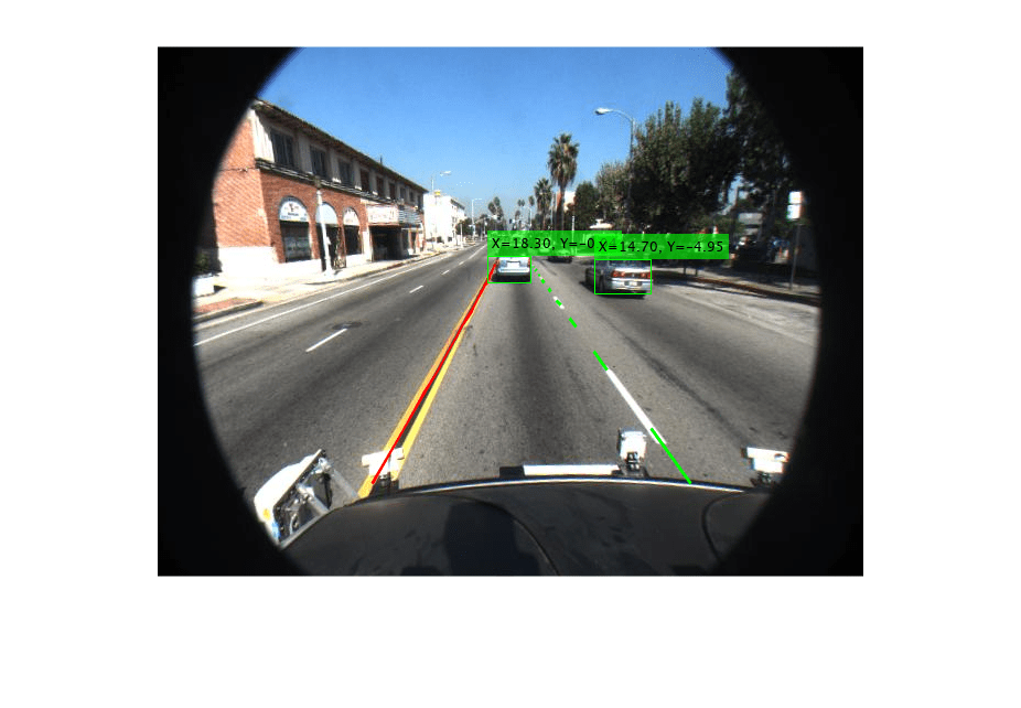
The example implements a subset of features found on a fully developed monocular camera system. It detects lane boundaries and backs of vehicles, and reports their locations in the vehicle coordinate system.

Define Camera Configuration

Knowing the camera's intrinsic and extrinsic calibration parameters is critical to accurate conversion between pixel and vehicle coordinates.

Start by defining the camera's intrinsic parameters. The parameters below were determined earlier using a camera calibration procedure that used a checkerboard calibration pattern. You can use the Camera Calibrator app to obtain them for your camera.

focalLength    = [309.4362, 344.2161]; % [fx, fy] in pixel units
principalPoint = [318.9034, 257.5352]; % [cx, cy] optical center in pixel coordinates
imageSize      = [480, 640];           % [nrows, mcols]

Note that the lens distortion coefficients were ignored, because there is little distortion in the data. The parameters are stored in a cameraIntrinsics object.

camIntrinsics = cameraIntrinsics(focalLength, principalPoint, imageSize);

Next, define the camera orientation with respect to the vehicle's chassis. You will use this information to establish camera extrinsics that define the position of the 3-D camera coordinate system with respect to the vehicle coordinate system.

height = 2.1798;    % mounting height in meters from the ground
pitch  = 14;        % pitch of the camera in degrees

The above quantities can be derived from the rotation and translation matrices returned by the estimateExtrinsics function. Pitch specifies the tilt of the camera from the horizontal position. For the camera used in this example, the roll and yaw of the sensor are both zero. The entire configuration defining the intrinsics and extrinsics is stored in the monoCamera object.

sensor = monoCamera(camIntrinsics, height, 'Pitch', pitch);

Note that the monoCamera object sets up a very specific vehicle coordinate system, where the X-axis points forward from the vehicle, the Y-axis points to the left of the vehicle, and the Z-axis points up from the ground.

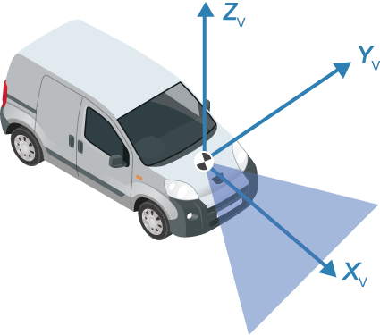
By default, the origin of the coordinate system is on the ground, directly below the camera center defined by the camera's focal point. When you wish to use another origin, the SensorLocation property of the monoCamera object can be used to give the camera's X and Y position relative to it. Additionally, monoCamera provides imageToVehicle and vehicleToImage methods for converting between image and vehicle coordinate systems.

Note: The conversion between the coordinate systems assumes a flat road. It is based on establishing a homography matrix that maps locations on the imaging plane to locations on the road surface. Nonflat roads introduce errors in distance computations, especially at locations that are far from the vehicle.

Load a Frame of Video

Before processing the entire video, process a single video frame to illustrate the concepts involved in the design of a monocular camera sensor.

Start by creating a VideoReader object that opens a video file. To be memory efficient, VideoReader loads one video frame at a time.

videoName = 'caltech_cordova1.avi';
videoReader = VideoReader(videoName);

Read an interesting frame that contains lane markers and a vehicle.

timeStamp = 0.06667;                   % time from the beginning of the video
videoReader.CurrentTime = timeStamp;   % point to the chosen frame

frame = readFrame(videoReader); % read frame at timeStamp seconds
imshow(frame) % display frame

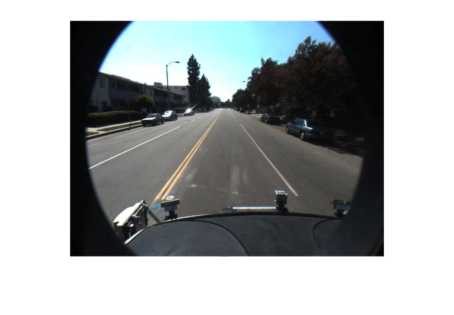
Note: This example ignores lens distortion. If you were concerned about errors in distance measurements introduced by the lens distortion, at this point you would use the undistortImage function to remove the lens distortion.

Create Bird's-Eye-View Image

There are many ways to segment and detect lane markers. One approach involves the use of a bird's-eye-view image transform. Although it incurs computational cost, this transform offers one major advantage. The lane markers in the bird's-eye view are of uniform thickness, thus simplifying the segmentation process. The lane markers belonging to the same lane also become parallel, thus making further analysis easier.

Given the camera setup, the birdsEyeView object transforms the original image to the bird's-eye view. This object lets you specify the area that you want to transform using vehicle coordinates. Note that the vehicle coordinate units were established by the monoCamera object, when the camera mounting height was specified in meters. For example, if the height was specified in millimeters, the rest of the simulation would use millimeters.

% Using vehicle coordinates, define area to transform
distAheadOfSensor = 30; % in meters, as previously specified in monoCamera height input
spaceToOneSide    = 6;  % all other distance quantities are also in meters
bottomOffset      = 3;

outView   = [bottomOffset, distAheadOfSensor, -spaceToOneSide, spaceToOneSide]; % [xmin, xmax, ymin, ymax]
imageSize = [NaN, 250]; % output image width in pixels; height is chosen automatically to preserve units per pixel ratio

birdsEyeConfig = birdsEyeView(sensor, outView, imageSize);

Generate bird's-eye-view image.

birdsEyeImage = transformImage(birdsEyeConfig, frame);
figure
imshow(birdsEyeImage)

The areas further away from the sensor are more blurry, due to having fewer pixels and thus requiring greater amount of interpolation.

Note that you can complete the latter processing steps without use of the bird's-eye view, as long as you can locate lane boundary candidate pixels in vehicle coordinates.

Find Lane Markers in Vehicle Coordinates

Having the bird's-eye-view image, you can now use the segmentLaneMarkerRidge function to separate lane marker candidate pixels from the road surface. This technique was chosen for its simplicity and relative effectiveness. Alternative segmentation techniques exist including semantic segmentation (deep learning) and steerable filters. You can substitute these techniques below to obtain a binary mask needed for the next stage.

Most input parameters to the functions below are specified in world units, for example, the lane marker width fed into segmentLaneMarkerRidge. The use of world units allows you to easily try new sensors, even when the input image size changes. This is very important to making the design more robust and flexible with respect to changing camera hardware and handling varying standards across many countries.

% Convert to grayscale
birdsEyeImage = im2gray(birdsEyeImage);

% Lane marker segmentation ROI in world units
vehicleROI = outView - [-1, 2, -3, 3]; % look 3 meters to left and right, and 4 meters ahead of the sensor
approxLaneMarkerWidthVehicle = 0.25; % 25 centimeters

% Detect lane features
laneSensitivity = 0.25;
birdsEyeViewBW = segmentLaneMarkerRidge(birdsEyeImage, birdsEyeConfig, approxLaneMarkerWidthVehicle,...
    'ROI', vehicleROI, 'Sensitivity', laneSensitivity);

figure
imshow(birdsEyeViewBW)

Locating individual lane markers takes place in vehicle coordinates that are anchored to the camera sensor. This example uses a parabolic lane boundary model, ax^2 + bx + c, to represent the lane markers. Other representations, such as a third-degree polynomial or splines, are possible. Conversion to vehicle coordinates is necessary, otherwise lane marker curvature cannot be properly represented by a parabola while it is affected by a perspective distortion.

The lane model holds for lane markers along a vehicle's path. Lane markers going across the path or road signs painted on the asphalt are rejected.

% Obtain lane candidate points in vehicle coordinates
[imageX, imageY] = find(birdsEyeViewBW);
xyBoundaryPoints = imageToVehicle(birdsEyeConfig, [imageY, imageX]);

Since the segmented points contain many outliers that are not part of the actual lane markers, use the robust curve fitting algorithm based on random sample consensus (RANSAC).

Return the boundaries and their parabola parameters (a, b, c) in an array of parabolicLaneBoundary objects, boundaries.

maxLanes      = 2; % look for maximum of two lane markers
boundaryWidth = 3*approxLaneMarkerWidthVehicle; % expand boundary width

[boundaries, boundaryPoints] = findParabolicLaneBoundaries(xyBoundaryPoints,boundaryWidth, ...
    'MaxNumBoundaries', maxLanes, 'validateBoundaryFcn', @validateBoundaryFcn);

Notice that the findParabolicLaneBoundaries takes a function handle, validateBoundaryFcn. This example function is listed at the end of this example. Using this additional input lets you reject some curves based on the values of the a, b, c parameters. It can also be used to take advantage of temporal information over a series of frames by constraining future a, b, c values based on previous video frames.

Determine Boundaries of the Ego Lane

Some of the curves found in the previous step might still be invalid. For example, when a curve is fit into crosswalk markers. Use additional heuristics to reject many such curves.

% Establish criteria for rejecting boundaries based on their length
maxPossibleXLength = diff(vehicleROI(1:2));
minXLength         = maxPossibleXLength * 0.60; % establish a threshold

% Find short boundaries
if( numel(boundaries) > 0 )
    isOfMinLength = false(1, numel(boundaries));
    for i = 1 : numel(boundaries)
        if(diff(boundaries(i).XExtent) > minXLength)
            isOfMinLength(i) = true;
        end
    end
else
    isOfMinLength = false;
end

Remove additional boundaries based on the strength metric computed by the findParabolicLaneBoundaries function. Set a lane strength threshold based on ROI and image size.

% To compute the maximum strength, assume all image pixels within the ROI
% are lane candidate points
birdsImageROI = vehicleToImageROI(birdsEyeConfig, vehicleROI);
[laneImageX,laneImageY] = meshgrid(birdsImageROI(1):birdsImageROI(2),birdsImageROI(3):birdsImageROI(4));

% Convert the image points to vehicle points
vehiclePoints = imageToVehicle(birdsEyeConfig,[laneImageX(:),laneImageY(:)]);

% Find the maximum number of unique x-axis locations possible for any lane
% boundary
maxPointsInOneLane = numel(unique(single((vehiclePoints(:,1)))));

% Set the maximum length of a lane boundary to the ROI length
maxLaneLength = diff(vehicleROI(1:2));

% Compute the maximum possible lane strength for this image size/ROI size
% specification
maxStrength   = maxPointsInOneLane/maxLaneLength;

% Reject short and weak boundaries
idx = 0;
strongBoundaries = parabolicLaneBoundary(zeros(nnz(isOfMinLength), 3));
for i = 1 : size(isOfMinLength,2)
    if( isOfMinLength(i) == 1 )
        if( boundaries(i).Strength > 0.4*maxStrength )
            idx = idx + 1;
            strongBoundaries(idx) = boundaries(i);
        end
    end
end

The heuristics to classify lane marker type as solid/dashed are included in a helper function listed at the bottom of this example. Knowing the lane marker type is critical for steering the vehicle automatically. For example, crossing a solid marker is prohibited.

% Classify lane marker type when boundaryPoints are not empty
if isempty(boundaryPoints)
    strongBoundaries = repmat(strongBoundaries,1,2);
    strongBoundaries(1) = parabolicLaneBoundary(zeros(1,3));
    strongBoundaries(2) = parabolicLaneBoundary(zeros(1,3));
else
    strongBoundaries = classifyLaneTypes(strongBoundaries, boundaryPoints);
end

distancesToBoundaries = coder.nullcopy(ones(size(strongBoundaries,2),1));

% Find ego lanes
xOffset    = 0;   %  0 meters from the sensor
for i = 1 : size(strongBoundaries, 2)
    distancesToBoundaries(i) = strongBoundaries(i).computeBoundaryModel(xOffset);
end

% Find candidate ego boundaries
distancesToLeftBoundary = distancesToBoundaries>0;
if (numel(distancesToBoundaries(distancesToLeftBoundary)))
    minLeftDistance = min(distancesToBoundaries(distancesToLeftBoundary));
else
    minLeftDistance = 0;
end

distancesToRightBoundary = (distancesToBoundaries <= 0);
if( numel(distancesToBoundaries(distancesToRightBoundary)))
    minRightDistance = max(distancesToBoundaries(distancesToRightBoundary));
else
    minRightDistance = 0;
end

% Find left ego boundary
if (minLeftDistance ~= 0)
    leftEgoBoundaryIndex  = distancesToBoundaries == minLeftDistance;
    leftEgoBoundary = parabolicLaneBoundary(zeros(nnz(leftEgoBoundaryIndex), 3));
    idx = 0;
    for i = 1 : size(leftEgoBoundaryIndex, 1)
        if( leftEgoBoundaryIndex(i) == 1)
            idx = idx + 1;
            leftEgoBoundary(idx) = strongBoundaries(i);
        end
    end
else
    leftEgoBoundary = parabolicLaneBoundary.empty();
end

% Find right ego boundary
if (minRightDistance ~= 0)
    rightEgoBoundaryIndex = distancesToBoundaries == minRightDistance;
    rightEgoBoundary = parabolicLaneBoundary(zeros(nnz(rightEgoBoundaryIndex), 3));
    idx = 0;
    for i = 1 : size(rightEgoBoundaryIndex, 1)
        if( rightEgoBoundaryIndex(i) == 1)
            idx = idx + 1;
            rightEgoBoundary(idx) = strongBoundaries(i);
        end
    end
else
    rightEgoBoundary = parabolicLaneBoundary.empty();
end

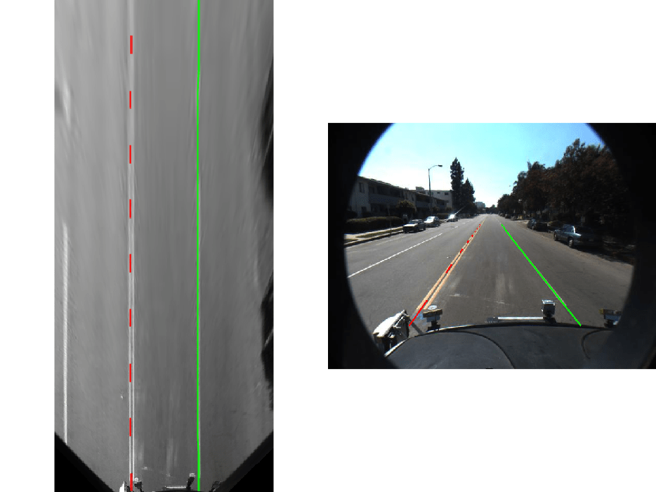
Show the detected lane markers in the bird's-eye-view image and in the regular view.

xVehiclePoints = bottomOffset:distAheadOfSensor;
birdsEyeWithEgoLane = insertLaneBoundary(birdsEyeImage, leftEgoBoundary , birdsEyeConfig, xVehiclePoints, 'Color','Red');
birdsEyeWithEgoLane = insertLaneBoundary(birdsEyeWithEgoLane, rightEgoBoundary, birdsEyeConfig, xVehiclePoints, 'Color','Green');

frameWithEgoLane = insertLaneBoundary(frame, leftEgoBoundary, sensor, xVehiclePoints, 'Color','Red');
frameWithEgoLane = insertLaneBoundary(frameWithEgoLane, rightEgoBoundary, sensor, xVehiclePoints, 'Color','Green');

figure
subplot('Position', [0, 0, 0.5, 1.0]) % [left, bottom, width, height] in normalized units
imshow(birdsEyeWithEgoLane)
subplot('Position', [0.5, 0, 0.5, 1.0])
imshow(frameWithEgoLane)

Locate Vehicles in Vehicle Coordinates

Detecting and tracking vehicles is critical in front collision warning (FCW) and autonomous emergency braking (AEB) systems.

Load an aggregate channel features (ACF) detector that is pretrained to detect the front and rear of vehicles. A detector like this can handle scenarios where issuing a collision warning is important. It is not sufficient, for example, for detecting a vehicle traveling across a road in front of the ego vehicle.

detector = vehicleDetectorACF();

% Width of a common vehicle is between 1.5 to 2.5 meters
vehicleWidth = [1.5, 2.5];

Use the configureDetectorMonoCamera function to specialize the generic ACF detector to take into account the geometry of the typical automotive application. By passing in this camera configuration, this new detector searches only for vehicles along the road's surface, because there is no point searching for vehicles high above the vanishing point. This saves computational time and reduces the number of false positives.

monoDetector = configureDetectorMonoCamera(detector, sensor, vehicleWidth);

[bboxes, scores] = detect(monoDetector, frame);

Because this example shows how to process only a single frame for demonstration purposes, you cannot apply tracking on top of the raw detections. The addition of tracking makes the results of returning vehicle locations more robust, because even when the vehicle is partly occluded, the tracker continues to return the vehicle's location. For more information, see the Track Multiple Vehicles Using a Camera example.

Next, convert vehicle detections to vehicle coordinates. The computeVehicleLocations function, included at the end of this example, calculates the location of a vehicle in vehicle coordinates given a bounding box returned by a detection algorithm in image coordinates. It returns the center location of the bottom of the bounding box in vehicle coordinates. Because we are using a monocular camera sensor and a simple homography, only distances along the surface of the road can be computed accurately. Computation of an arbitrary location in 3-D space requires use of stereo camera or another sensor capable of triangulation.

locations = computeVehicleLocations(bboxes, sensor);

% Overlay the detections on the video frame
imgOut = insertVehicleDetections(frame, locations, bboxes);
figure;
imshow(imgOut);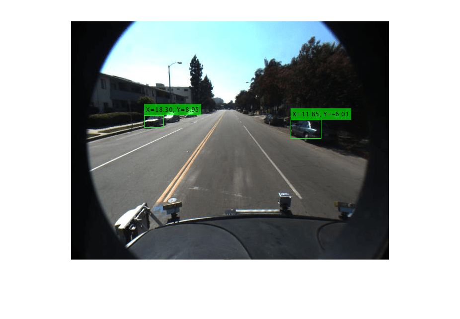

Simulate a Complete Sensor with Video Input

Now that you have an idea about the inner workings of the individual steps, let's put them together and apply them to a video sequence where we can also take advantage of temporal information.

Rewind the video to the beginning, and then process the video. The code below is shortened because all the key parameters were defined in the previous steps. Here, the parameters are used without further explanation.

videoReader.CurrentTime = 0;

isPlayerOpen = true;
snapshot     = [];
while hasFrame(videoReader) && isPlayerOpen
   
    % Grab a frame of video
    frame = readFrame(videoReader);
    
    % Compute birdsEyeView image
    birdsEyeImage = transformImage(birdsEyeConfig, frame);
    birdsEyeImage = im2gray(birdsEyeImage);
    
    % Detect lane boundary features
    birdsEyeViewBW = segmentLaneMarkerRidge(birdsEyeImage, birdsEyeConfig, ...
        approxLaneMarkerWidthVehicle, 'ROI', vehicleROI, ...
        'Sensitivity', laneSensitivity);

    % Obtain lane candidate points in vehicle coordinates
    [imageX, imageY] = find(birdsEyeViewBW);
    xyBoundaryPoints = imageToVehicle(birdsEyeConfig, [imageY, imageX]);

    % Find lane boundary candidates
    [boundaries, boundaryPoints] = findParabolicLaneBoundaries(xyBoundaryPoints,boundaryWidth, ...
        'MaxNumBoundaries', maxLanes, 'validateBoundaryFcn', @validateBoundaryFcn);
    
    % Reject boundaries based on their length and strength    
    % Find short boundaries
    if( numel(boundaries) > 0 )
        isOfMinLength = false(1, numel(boundaries));
        for i = 1 : numel(boundaries)
            if(diff(boundaries(i).XExtent) > minXLength)
                isOfMinLength(i) = true;
            end
        end
    else
        isOfMinLength = false;
    end

    % Reject short and weak boundaries
    idx = 0;
    strongBoundaries = parabolicLaneBoundary(zeros(nnz(isOfMinLength), 3));
    for i = 1 : size(isOfMinLength,2)
        if( isOfMinLength(i) == 1 )
            if( boundaries(i).Strength > 0.2*maxStrength )
                idx = idx + 1;
                strongBoundaries(idx) = boundaries(i);
            end
        end
    end

    boundaries    = boundaries(isOfMinLength);
    isStrong      = [boundaries.Strength] > 0.2*maxStrength;
    boundaries    = boundaries(isStrong);

    % Classify lane marker type when boundaryPoints are not empty
    if isempty(boundaryPoints)
        strongBoundaries = repmat(strongBoundaries,1,2);
        strongBoundaries(1) = parabolicLaneBoundary(zeros(1,3));
        strongBoundaries(2) = parabolicLaneBoundary(zeros(1,3));
    else
        strongBoundaries = classifyLaneTypes(strongBoundaries, boundaryPoints);
    end     
        
    % Find ego lanes
    xOffset    = 0;   %  0 meters from the sensor
    distancesToBoundaries = coder.nullcopy(ones(size(strongBoundaries,2),1));

    for i = 1 : size(strongBoundaries, 2)
        distancesToBoundaries(i) = strongBoundaries(i).computeBoundaryModel(xOffset);
    end
    % Find candidate ego boundaries
    distancesToLeftBoundary = distancesToBoundaries>0;
    if (numel(distancesToBoundaries(distancesToLeftBoundary)))
        minLeftDistance = min(distancesToBoundaries(distancesToLeftBoundary));
    else
        minLeftDistance = 0;
    end

    distancesToRightBoundary = (distancesToBoundaries <= 0);
    if( numel(distancesToBoundaries(distancesToRightBoundary)))
        minRightDistance = max(distancesToBoundaries(distancesToRightBoundary));
    else
        minRightDistance = 0;
    end

    % Find left ego boundary
    if (minLeftDistance ~= 0)
        leftEgoBoundaryIndex  = distancesToBoundaries == minLeftDistance;
        leftEgoBoundary = parabolicLaneBoundary(zeros(nnz(leftEgoBoundaryIndex), 3));
        idx = 0;
        for i = 1 : size(leftEgoBoundaryIndex, 1)
            if( leftEgoBoundaryIndex(i) == 1)
                idx = idx + 1;
                leftEgoBoundary(idx) = strongBoundaries(i);
            end
        end
    else
        leftEgoBoundary = parabolicLaneBoundary.empty();
    end
    % Find right ego boundary
    if (minRightDistance ~= 0)
        rightEgoBoundaryIndex = distancesToBoundaries == minRightDistance;
        rightEgoBoundary = parabolicLaneBoundary(zeros(nnz(rightEgoBoundaryIndex), 3));
        idx = 0;
        for i = 1 : size(rightEgoBoundaryIndex, 1)
            if( rightEgoBoundaryIndex(i) == 1)
                idx = idx + 1;
                rightEgoBoundary(idx) = strongBoundaries(i);
            end
        end
    else
        rightEgoBoundary = parabolicLaneBoundary.empty();
    end

    
    % Detect vehicles
    [bboxes, scores] = detect(monoDetector, frame);
    locations = computeVehicleLocations(bboxes, sensor);
    
    % Visualize sensor outputs and intermediate results. Pack the core
    % sensor outputs into a struct.
    sensorOut.leftEgoBoundary  = leftEgoBoundary;
    sensorOut.rightEgoBoundary = rightEgoBoundary;
    sensorOut.vehicleLocations = locations;
    
    sensorOut.xVehiclePoints   = bottomOffset:distAheadOfSensor;
    sensorOut.vehicleBoxes     = bboxes;
    
    % Pack additional visualization data, including intermediate results
    intOut.birdsEyeImage   = birdsEyeImage;    
    intOut.birdsEyeConfig  = birdsEyeConfig;
    intOut.vehicleScores   = scores;
    intOut.vehicleROI      = vehicleROI;
    intOut.birdsEyeBW      = birdsEyeViewBW;
    
    closePlayers = ~hasFrame(videoReader);
    isPlayerOpen = visualizeSensorResults(frame, sensor, sensorOut, ...
        intOut, closePlayers);
    
    timeStamp = 7.5333; % take snapshot for publishing at timeStamp seconds
    if abs(videoReader.CurrentTime - timeStamp) < 0.01
        snapshot = takeSnapshot(frame, sensor, sensorOut);
    end    
end

Display the video frame. Snapshot is taken at timeStamp seconds.

if ~isempty(snapshot)
    figure
    imshow(snapshot)
end

Try the Sensor Design on a Different Video

The helperMonoSensor class assembles the setup and all the necessary steps to simulate the monocular camera sensor into a complete package that can be applied to any video. Since most parameters used by the sensor design are based on world units, the design is robust to changes in camera parameters, including the image size. Note that the code inside the helperMonoSensor class is different from the loop in the previous section, which was used to illustrate basic concepts.

Besides providing a new video, you must supply a camera configuration corresponding to that video. The process is shown here. Try it on your own videos.

% Sensor configuration
focalLength    = [309.4362, 344.2161];
principalPoint = [318.9034, 257.5352];
imageSize      = [480, 640];
height         = 2.1798;    % mounting height in meters from the ground
pitch          = 14;        % pitch of the camera in degrees

camIntrinsics = cameraIntrinsics(focalLength, principalPoint, imageSize);
sensor        = monoCamera(camIntrinsics, height, 'Pitch', pitch);

videoReader = VideoReader('caltech_washington1.avi');

Create the helperMonoSensor object and apply it to the video.

monoSensor   = helperMonoSensor(sensor);
monoSensor.LaneXExtentThreshold = 0.5;
% To remove false detections from shadows in this video, we only return
% vehicle detections with higher scores.
monoSensor.VehicleDetectionThreshold = 20;    

isPlayerOpen = true;
snapshot     = [];
while hasFrame(videoReader) && isPlayerOpen
    
    frame = readFrame(videoReader); % get a frame
    
    sensorOut = processFrame(monoSensor, frame);

    closePlayers = ~hasFrame(videoReader);
            
    isPlayerOpen = displaySensorOutputs(monoSensor, frame, sensorOut, closePlayers);
    
    timeStamp = 11.1333; % take snapshot for publishing at timeStamp seconds
    if abs(videoReader.CurrentTime - timeStamp) < 0.01
        snapshot = takeSnapshot(frame, sensor, sensorOut);
    end
   
end

Display the video frame. Snapshot is taken at timeStamp seconds.

if ~isempty(snapshot)
    figure
    imshow(snapshot)
end

Supporting Functions

visualizeSensorResults displays core information and intermediate results from the monocular camera sensor simulation.

function isPlayerOpen = visualizeSensorResults(frame, sensor, sensorOut,...
    intOut, closePlayers)

    % Unpack the main inputs
    leftEgoBoundary  = sensorOut.leftEgoBoundary;
    rightEgoBoundary = sensorOut.rightEgoBoundary;
    locations        = sensorOut.vehicleLocations;

    xVehiclePoints   = sensorOut.xVehiclePoints;    
    bboxes           = sensorOut.vehicleBoxes;
    
    % Unpack additional intermediate data
    birdsEyeViewImage = intOut.birdsEyeImage;
    birdsEyeConfig          = intOut.birdsEyeConfig;
    vehicleROI        = intOut.vehicleROI;
    birdsEyeViewBW    = intOut.birdsEyeBW;
    
    % Visualize left and right ego-lane boundaries in bird's-eye view
    birdsEyeWithOverlays = insertLaneBoundary(birdsEyeViewImage, leftEgoBoundary , birdsEyeConfig, xVehiclePoints, 'Color','Red');
    birdsEyeWithOverlays = insertLaneBoundary(birdsEyeWithOverlays, rightEgoBoundary, birdsEyeConfig, xVehiclePoints, 'Color','Green');
    
    % Visualize ego-lane boundaries in camera view
    frameWithOverlays = insertLaneBoundary(frame, leftEgoBoundary, sensor, xVehiclePoints, 'Color','Red');
    frameWithOverlays = insertLaneBoundary(frameWithOverlays, rightEgoBoundary, sensor, xVehiclePoints, 'Color','Green');

    frameWithOverlays = insertVehicleDetections(frameWithOverlays, locations, bboxes);

    imageROI = vehicleToImageROI(birdsEyeConfig, vehicleROI);
    ROI = [imageROI(1) imageROI(3) imageROI(2)-imageROI(1) imageROI(4)-imageROI(3)];

    % Highlight candidate lane points that include outliers
    birdsEyeViewImage = insertShape(birdsEyeViewImage, 'rectangle', ROI); % show detection ROI
    birdsEyeViewImage = imoverlay(birdsEyeViewImage, birdsEyeViewBW, 'blue');
        
    % Display the results
    frames = {frameWithOverlays, birdsEyeViewImage, birdsEyeWithOverlays};
    
    persistent players;
    if isempty(players)
        frameNames = {'Lane marker and vehicle detections', 'Raw segmentation', 'Lane marker detections'};
        players = helperVideoPlayerSet(frames, frameNames);
    end    
    update(players, frames);
    
    % Terminate the loop when the first player is closed
    isPlayerOpen = isOpen(players, 1);
    
    if (~isPlayerOpen || closePlayers) % close down the other players
        clear players;
    end
end

computeVehicleLocations calculates the location of a vehicle in vehicle coordinates, given a bounding box returned by a detection algorithm in image coordinates. It returns the center location of the bottom of the bounding box in vehicle coordinates. Because a monocular camera sensor and a simple homography are used, only distances along the surface of the road can be computed. Computation of an arbitrary location in 3-D space requires use of a stereo camera or another sensor capable of triangulation.

function locations = computeVehicleLocations(bboxes, sensor)

locations = zeros(size(bboxes,1),2);
for i = 1:size(bboxes, 1)
    bbox  = bboxes(i, :);
    
    % Get [x,y] location of the center of the lower portion of the
    % detection bounding box in meters. bbox is [x, y, width, height] in
    % image coordinates, where [x,y] represents upper-left corner.
    yBottom = bbox(2) + bbox(4) - 1;
    xCenter = bbox(1) + (bbox(3)-1)/2; % approximate center
    
    locations(i,:) = imageToVehicle(sensor, [xCenter, yBottom]);
end
end

insertVehicleDetections inserts bounding boxes and displays [x,y] locations corresponding to returned vehicle detections.

function imgOut = insertVehicleDetections(imgIn, locations, bboxes)

imgOut = imgIn;

for i = 1:size(locations, 1)
    location = locations(i, :);
    bbox     = bboxes(i, :);
        
    label = sprintf('X=%0.2f, Y=%0.2f', location(1), location(2));

    imgOut = insertObjectAnnotation(imgOut, ...
        'rectangle', bbox, label, 'AnnotationColor','g');
end
end

vehicleToImageROI converts ROI in vehicle coordinates to image coordinates in bird's-eye-view image.

function imageROI = vehicleToImageROI(birdsEyeConfig, vehicleROI)

vehicleROI = double(vehicleROI);

loc2 = abs(vehicleToImage(birdsEyeConfig, [vehicleROI(2) vehicleROI(4)]));
loc1 = abs(vehicleToImage(birdsEyeConfig, [vehicleROI(1) vehicleROI(4)]));
loc4 =     vehicleToImage(birdsEyeConfig, [vehicleROI(1) vehicleROI(4)]);
loc3 =     vehicleToImage(birdsEyeConfig, [vehicleROI(1) vehicleROI(3)]);

[minRoiX, maxRoiX, minRoiY, maxRoiY] = deal(loc4(1), loc3(1), loc2(2), loc1(2));

imageROI = round([minRoiX, maxRoiX, minRoiY, maxRoiY]);

end

validateBoundaryFcn rejects some of the lane boundary curves computed using the RANSAC algorithm.

function isGood = validateBoundaryFcn(params)

if ~isempty(params)
    a = params(1);
    
    % Reject any curve with a small 'a' coefficient, which makes it highly
    % curved.
    isGood = abs(a) < 0.003; % a from ax^2+bx+c
else
    isGood = false;
end
end

classifyLaneTypes determines lane marker types as solid, dashed, etc.

function boundaries = classifyLaneTypes(boundaries, boundaryPoints)

for bInd = 1 : size(boundaries,2)

    vehiclePoints = boundaryPoints{bInd};
    % Sort by x
    vehiclePoints = sortrows(vehiclePoints, 1);

    xVehicle = vehiclePoints(:,1);
    xVehicleUnique = unique(xVehicle);

    % Dashed vs solid
    xdiff  = diff(xVehicleUnique);
    % Set a threshold to remove gaps in solid line but not the spaces from
    % dashed lines.
    xdiffThreshold = mean(xdiff) + 3*std(xdiff);
    largeGaps = xdiff(xdiff > xdiffThreshold);

    % Safe default
    boundary = boundaries(bInd);           % changed according to set/get methods
    boundary.BoundaryType= LaneBoundaryType.Solid;

    if largeGaps>1
        % Ideally, these gaps should be consistent, but you cannot rely
        % on that unless you know that the ROI extent includes at least 3 dashes.
        boundary.BoundaryType= LaneBoundaryType.Dashed;
    end
    boundaries(bInd) = boundary;
end
end

takeSnapshot captures the output for the HTML publishing report.

function I = takeSnapshot(frame, sensor, sensorOut)

    % Unpack the inputs
    leftEgoBoundary  = sensorOut.leftEgoBoundary;
    rightEgoBoundary = sensorOut.rightEgoBoundary;
    locations        = sensorOut.vehicleLocations;
    xVehiclePoints   = sensorOut.xVehiclePoints;
    bboxes           = sensorOut.vehicleBoxes;
      
    frameWithOverlays = insertLaneBoundary(frame, leftEgoBoundary, sensor, xVehiclePoints, 'Color','Red');
    frameWithOverlays = insertLaneBoundary(frameWithOverlays, rightEgoBoundary, sensor, xVehiclePoints, 'Color','Green');
    frameWithOverlays = insertVehicleDetections(frameWithOverlays, locations, bboxes);
   
    I = frameWithOverlays;

end