Investigate Classification Decisions Using Gradient Attribution Techniques

This example shows how to use gradient attribution maps to investigate which parts of an image are most important for classification decisions made by a deep neural network.

Deep neural networks can look like black box decision makers — they give excellent results on complex problems, but it can be hard to understand why a network gives a particular output. Explainability is increasingly important as deep networks are used in more applications. To consider a network explainable, it must be clear what parts of the input data the network is using to make a decision and how much this data contributes to the network output.

A range of visualization techniques are available to determine if a network is using sensible parts of the input data to make a classification decision. As well as the gradient attribution methods shown in this example, you can use techniques such as gradient-weighted class-activation mapping (Grad-CAM) and occlusion sensitivity. For examples, see

• Understand Network Predictions Using Occlusion

• Grad-CAM Reveals the Why Behind Deep Learning Decisions

The gradient attribution methods explored in this example provide pixel-resolution maps that show which pixels are most important to the network's classification. They compute the gradient of the class score with respect to the input pixels. Intuitively, the map shows which pixels most affect the class score when changed. The gradient attribution methods produce maps with higher resolution than those from Grad-CAM or occlusion sensitivity, but that tend to be much noisier, as a well-trained deep network is not strongly dependent on the exact value of specific pixels. Use the gradient attribution techniques to find the broad areas of an image that are important to the classification.

The simplest gradient attribution map is the gradient of the class score for the predicted class with respect to each pixel in the input image [1]. This shows which pixels have the largest impact on the class score, and therefore which pixels are most important to the classification. This example shows how to use gradient attribution and two extended methods: guided backpropagation [2] and integrated gradients [3]. The use of these techniques is under debate as it is not clear how much insight these extensions can provide into the model [4].

Load Pretrained Network and Image

Load the pretrained GoogLeNet network.

net = googlenet;

Extract the image input size and the output classes of the network.

inputSize = net.Layers(1).InputSize(1:2);
classes = net.Layers(end).Classes;

Load the image. The image is of a dog named Laika. Resize the image to the network input size.

img = imread("laika_grass.jpg");
img = imresize(img,inputSize);

Classify the image and display the predicted class and classification score.

[YPred, scores] = classify(net, img);
[score, classIdx] = max(scores);

predClass = classes(classIdx);

imshow(img);
title(sprintf("%s (%.2f)",string(predClass),s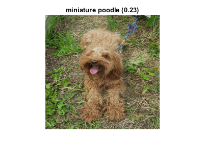core));

The network classifies Laika as a miniature poodle, which is a reasonable guess. She is a poodle/cocker spaniel cross.

Compute Gradient Attribution Map Using Automatic Differentiation

The gradient attribution techniques rely on finding the gradient of the prediction score with respect to the input image. The gradient attribution map is calculated using the following formula:

$${\mathit{W}}_{\mathrm{xy}}^{\mathit{c}}=\frac{\partial {\mathit{S}}^{\mathit{c}}}{\partial {\mathit{I}}_{\mathrm{xy}}}$$

where ${\mathit{W}}_{\mathrm{xy}}^{\mathit{c}}$ represents the importance of the pixel at location $\left(\mathit{x},\mathit{y}\right)$ to the prediction of class $\mathit{c}$, ${\mathit{S}}^{\mathit{c}}$ is the softmax score for that class, and ${\mathit{I}}_{\mathrm{xy}}$ is the image at pixel location $\left(\mathit{x},\mathit{y}\right)$ [1].

Convert the network to a dlnetwork so that you can use automatic differentiation to compute the gradients.

lgraph = layerGraph(net);
lgraph = removeLayers(lgraph,lgraph.Layers(end).Name);

dlnet = dlnetwork(lgraph);

Specify the name of the softmax layer, 'prob'.

softmaxName = 'prob';

To use automatic differentiation, convert the image of Laika to a dlarray.

dlImg = dlarray(single(img),'SSC');

Use dlfeval and the gradientMap function (defined in the Supporting Functions section of this example) to compute the derivative $\frac{\partial {\mathit{S}}^{\mathit{c}}}{\partial {\mathit{I}}_{\mathrm{xy}}}$. The gradientMap function passes the image forward through the network to obtain the class scores and contains a call to dlgradient to evaluate the gradients of the scores with respect to the image.

dydI = dlfeval(@gradientMap,dlnet,dlImg,softmaxName,classIdx);

The attribution map dydI is a 227-by-227-by-3 array. Each element in each channel corresponds to the gradient of the class score with respect to the input image for that channel of the original RGB image.

There are a number of ways to visualize this map. Directly plotting the gradient attribution map as an RGB image can be unclear as the map is typically quite noisy. Instead, sum the absolute values of each pixel along the channel dimension, then rescale between 0 and 1. Display the gradient attribution map using a custom colormap with 255 colors that maps values of 0 to white and 1 to black.

map = sum(abs(extractdata(dydI)),3);
map = rescale(map);

cmap = [linspace(1,0,255)' linspace(1,0,255)' linspace(1,0,255)'];

imshow(map, "Colormap", cmap);
title("Gradient Attribution Map (" + string(predClass) + ")");

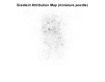
The darkest parts of the map are those centered around the dog. The map is extremely noisy, but it does suggest that the network is using the expected information in the image to perform classification. The pixels in the dog have much more impact on the classification score than the pixels of the grassy background.

Sharpen the Gradient Attribution Map Using Guided Backpropagation

You can obtain a sharper gradient attribution map by modifying the network's backwards pass through ReLU layers so that elements of the gradient that are less than zero and elements of the input to the ReLU layer that are less than zero are both set to zero. This is known as guided backpropagation [2].

The guided backpropagation backward function is:

$$\frac{\mathrm{dL}}{\mathrm{dZ}}=\left(\mathit{X}>0\right)*\left(\frac{\mathrm{dL}}{\mathrm{dZ}}>0\right)*\frac{\mathrm{dL}}{\mathrm{dZ}}$$

where $\mathit{L}$ is the loss, $\mathit{X}$ is the input to the ReLU layer, and $\mathit{Z}$ is the output.

You can write a custom layer with a non-standard backward pass, and use it with automatic differentiation. A custom layer class CustomBackpropReluLayer that implements this modification is included as a supporting file in this example. When automatic differentiation backpropagates through CustomBackpropReluLayer objects, it uses the modified guided backpropagation function defined in the custom layer.

Use the supporting function replaceLayersOfType (defined in the Supporting Functions section of this example) to replace all instances of reluLayer in the network with instances of CustomBackpropReluLayer. Set the BackpropMode property of each CustomBackpropReluLayer to "guided-backprop".

customRelu = CustomBackpropReluLayer();
customRelu.BackpropMode = "guided-backprop";

lgraphGB = replaceLayersOfType(lgraph, ...
    "nnet.cnn.layer.ReLULayer",customRelu);

Convert the layer graph containing the CustomBackpropReluLayers into a dlnetwork.

dlnetGB = dlnetwork(lgraphGB);

Compute and plot the gradient attribution map for the network using guided backpropagation.

dydIGB = dlfeval(@gradientMap,dlnetGB,dlImg,softmaxName,classIdx);

mapGB = sum(abs(extractdata(dydIGB)),3);
mapGB = rescale(mapGB);

imshow(mapGB, "Colormap", cmap);
title("Guided Backpropagation (" + string(predClass) + ")");

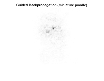
You can see that guided backpropagation technique more clearly highlights different parts of the dog, such as the eyes and nose.

You can also use the Zeiler-Fergus technique for backpropagation through ReLU layers [5]. For the Zeiler-Fergus technique, the backward function is given as:

$$\frac{\mathrm{dL}}{\mathrm{dZ}}=\left(\frac{\mathrm{dL}}{\mathrm{dZ}}>0\right)*\frac{\mathrm{dL}}{\mathrm{dZ}}$$

Set the BackpropMode property of the CustomBackpropReluLayer instances to "zeiler-fergus".

customReluZF = CustomBackpropReluLayer();
customReluZF.BackpropMode = "zeiler-fergus";

lgraphZF = replaceLayersOfType(lgraph, ...
    "nnet.cnn.layer.ReLULayer",customReluZF);

dlnetZF = dlnetwork(lgraphZF);

dydIZF = dlfeval(@gradientMap,dlnetZF,dlImg,softmaxName,classIdx);


mapZF = sum(abs(extractdata(dydIZF)),3);
mapZF = rescale(mapZF);

imshow(mapZF,"Colormap", cmap);
title("Zeiler-Fergus (" + string(predClass) + ")");

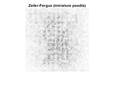
The gradient attribution maps computed using the Zeiler-Fergus backpropagation technique are much less clear than those computed using guided backpropagation.

Evaluate Sensitivity to Image Changes Using Integrated Gradients

The integrated gradients approach computes integrates the gradients of class score with respect to image pixels across a set of images that are linearly interpolated between a baseline image and the original image of interest [3]. The integrated gradients technique is designed to be sensitive to the changes in the pixel value over the integration, such that if a change in a pixel value affects the class score, that pixel has a non-zero value in the map. Non-linearities in the network, such as ReLU layers, can prevent this sensitivity in simpler gradient attribution techniques.

The integrated gradients attribution map is calculated as

${\mathit{W}}_{\mathrm{xy}}^{\mathit{c}}=\left({\mathit{I}}_{\mathrm{xy}}-{\mathit{I}}_{\mathrm{xy}}^0\right){\int }_{\alpha =0}^1\mathit{d}\alpha \frac{\partial {\mathit{S}}^{\mathit{c}}\left({\mathit{I}}_{\mathrm{xy}}\left(\alpha \right)\right)}{\partial {\mathit{I}}_{\mathrm{xy}}\left(\alpha \right)}$,

where ${\mathit{W}}_{\mathrm{xy}}^{\mathit{c}}$ is the map's value for class $\mathit{c}$ at pixel location $\left(\mathit{x},\mathit{y}\right)$, ${\mathit{I}}_{\mathrm{xy}}^0$ is a baseline image, and ${\mathit{I}}_{\mathrm{xy}}\left(\alpha \right)$ is the image at a distance $\alpha$ along the path between the baseline image and the input image:

${\mathit{I}}_{\mathrm{xy}}\left(\alpha \right)={\mathit{I}}_{\mathrm{xy}}^0+\alpha \left({\mathit{I}}_{\mathrm{xy}}-{\mathit{I}}_{\mathrm{xy}}^0\right)$.

In this example, the integrated gradients formula is simplified by summing over a discrete index,$\mathit{n}$, instead of integrating over $\alpha$:

${\mathit{W}}_{\mathrm{xy}}^{\mathit{c}}=\left({\mathit{I}}_{\mathrm{xy}}-{\mathit{I}}_{\mathrm{xy}}^0\right)\sum _{\mathit{n}=0}^{\mathit{N}}\frac{\partial {\mathit{S}}^{\mathit{c}}\left({\mathit{I}}_{\mathrm{xy}}^{\mathit{n}}\right)}{\partial {\mathit{I}}_{\mathrm{xy}}^{\mathit{n}}}$,

with

${\mathit{I}}_{\mathrm{xy}}^{\mathit{n}}={\mathit{I}}_{\mathrm{xy}}^0+\frac{\mathit{n}}{\mathit{N}}\left({\mathit{I}}_{\mathrm{xy}}-{\mathit{I}}_{\mathrm{xy}}^0\right)$.

For image data, choose the baseline image to be a black image of zeros. Find the image that is the difference between the original image and the baseline image. In this case, differenceImg is the same as the original image as the baseline image is zero.

baselineImg = zeros([inputSize, 3]);
differenceImg = single(img) - baselineImg;

Create an array of images corresponding to discrete steps along the linear path from the baseline image to the original input image. A larger number of images will give smoother results but take longer to compute.

numPathImages = 25;

pathImgs = zeros([inputSize 3 numPathImages-1]);
for n=0:numPathImages-1
    pathImgs(:,:,:,n+1) = baselineImg + (n)/(numPathImages-1) * differenceImg;
end

figure;
imshow(imtile(rescale(pathImgs)));
title("Images Along Integration Path");

Convert the mini-batch of path images to a dlarray. Format the data with the format 'SSCB' for the two spatial, one channel and one batch dimensions. Each path image is a single observation in the mini-batch. Compute the gradient map for the resulting batch of images along the path.

dlPathImgs = dlarray(pathImgs, 'SSCB');
dydIIG = dlfeval(@gradientMap, dlnet, dlPathImgs, softmaxName, classIdx);

For each channel, sum the gradients of all observations in the mini-batch.

dydIIGSum = sum(dydIIG,4);

Multiply each element of the summed gradient attribution maps with the corresponding element of differenceImg. To compute the integrated gradient attribution map, sum over each channel and rescale.

dydIIGSum = differenceImg .* dydIIGSum;

mapIG = sum(extractdata(abs(dydIIGSum)),3);
mapIG = rescale(mapIG);

imshow(mapIG, "Colormap", cmap);
title("Integrated Gradients (" + string(predClass) + ")");

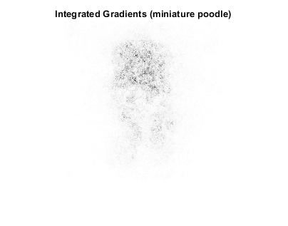
The computed map shows the network is more strongly focused on the dog's face as a means of deciding on its class.

The gradient attribution techniques demonstrated here can be used to check whether your network is focusing on the expected parts of the image when making a classification. To get good insights into the way your model is working and explain classification decisions, you can perform these techniques on a range of images and find the specific features that strongly contribute to a particular class. The unmodified gradient attributions technique is likely to be the more reliable method for explaining network decisions. While the guided backpropagation and integrated gradient techniques can produce the clearest gradient maps, it is not clear how much insight these techniques can provide into how the model works [4].

Supporting Functions

Gradient Map Function

The function gradientMap computes the gradients of the score with respect to an image, for a specified class. The function accepts a single image or a mini-batch of images. Within this example, the function gradientMap is introduced in the section Compute Gradient Attribution Map Using Automatic Differentiation.

function dydI = gradientMap(dlnet, dlImgs, softmaxName, classIdx)
% Compute the gradient of a class score with respect to one or more input
% images.

dydI = dlarray(zeros(size(dlImgs)));

for i=1:size(dlImgs,4)
    I = dlImgs(:,:,:,i);
    scores = predict(dlnet,I,'Outputs',{softmaxName});
    classScore = scores(classIdx);
    dydI(:,:,:,i) = dlgradient(classScore,I);
end
end

Replace Layers Function

The replaceLayersOfType function replaces all layers of the specified class with instances of a new layer. The new layers are named with the same names as the original layers. Within this example, the function replaceLayersOfType is introduced in the section Sharpen the Gradient Attribution Map using Guided Backpropagation.

function lgraph = replaceLayersOfType(lgraph, layerType, newLayer)
% Replace layers in the layerGraph lgraph of the type specified by
% layerType with copies of the layer newLayer.

for i=1:length(lgraph.Layers)
    if isa(lgraph.Layers(i), layerType)
        % Match names between old and new layer.
        layerName = lgraph.Layers(i).Name;
        newLayer.Name = layerName;
        
        lgraph = replaceLayer(lgraph, layerName, newLayer);
    end
end
end

References

[1] Simonyan, Karen, Andrea Vedaldi, and Andrew Zisserman. “Deep Inside Convolutional Networks: Visualising Image Classification Models and Saliency Maps.” ArXiv:1312.6034 [Cs], April 19, 2014. http://arxiv.org/abs/1312.6034.

[2] Springenberg, Jost Tobias, Alexey Dosovitskiy, Thomas Brox, and Martin Riedmiller. “Striving for Simplicity: The All Convolutional Net.” ArXiv:1412.6806 [Cs], April 13, 2015. http://arxiv.org/abs/1412.6806.

[3] Sundararajan, Mukund, Ankur Taly, and Qiqi Yan. "Axiomatic Attribution for Deep Networks." Proceedings of the 34th International Conference on Machine Learning (PMLR) 70 (2017): 3319-3328

[4] Adebayo, Julius, Justin Gilmer, Michael Muelly, Ian Goodfellow, Moritz Hardt, and Been Kim. “Sanity Checks for Saliency Maps.” ArXiv:1810.03292 [Cs, Stat], October 27, 2018. http://arxiv.org/abs/1810.03292.

[5] Zeiler, Matthew D. and Rob Fergus. "Visualizing and Understanding Convolutional Networks." In Computer Vision – ECCV 2014. Lecture Notes in Computer Science 8689, edited by D. Fleet, T. Pajdla, B. Schiele, T. Tuytelaars. Springer, Cham, 2014.