Linear System Analyzer
Analyze time-domain and frequency-domain responses of linear time-invariant (LTI) systems
Description
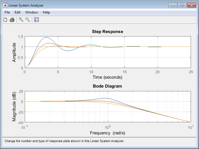
The Linear System Analyzer app lets you analyze time-domain and frequency-domain responses of LTI systems.
Using this app, you can:
View and compare the response plots of SISO and MIMO systems or of several linear models at the same time.
Generate time response plots such as step, impulse, and time response to arbitrary inputs.
Generate frequency response plots such as Bode, Nyquist, Nichols, singular-value, and pole-zero plots.
Inspect key response characteristics, such as rise time, maximum overshoot, and stability margins.
Linear System Analyzer can generate the following response plots:
Step response
Impulse response
Simulated time response to specified input signal
Simulated time response from specified initial conditions (state-space models only)
Bode diagram (magnitude and phase, or magnitude alone)
Nyquist plot
Nichols plot
Singular value plot
Pole/zero map and I/O pole/zero map
Open the Linear System Analyzer App
MATLAB® Toolstrip: On the Apps tab, under Control System Design and Analysis, click the app icon.
MATLAB command prompt: Enter
linearSystemAnalyzer.
Examples
To import models into Linear System Analyzer, select File > Import. The Import System Data dialog box opens.
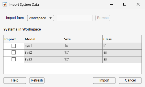
Under Import from, select whether to import a model from:
The MATLAB workspace by selecting
WorkspaceA MAT-file by selecting
MAT-file
In the Import column of the table, select one or models to import.
Click the Import.
To export models from Linear System Analyzer, select File > Export. The Linear System Analyzer Export dialog box opens.
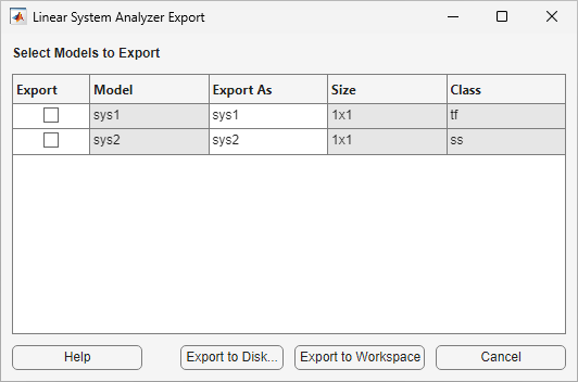
In the Export column of the table, select one or models to import.
To export models to the MATLAB workspace, click Export to Workspace.
To export models to a MAT-file, click Export to Disk.
In the Select File to Write dialog box, specify the name and location for saved MAT-file and click Save.
To remove models from Linear System Analyzer, select Edit > Delete Systems. The Linear System Analyzer Delete dialog box opens.
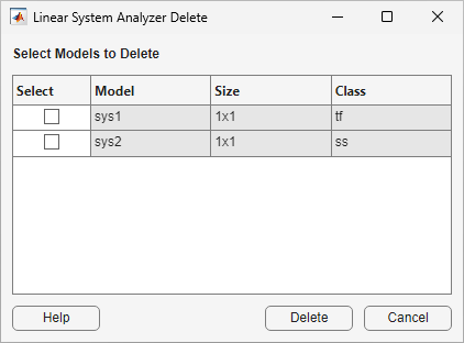
In the Select column, select one or models to delete.
Click Delete.
To interactively specify the types of responses to plot, in Linear System Analyzer, select Edit > Plot Configurations. The Plot Configurations dialog box opens.
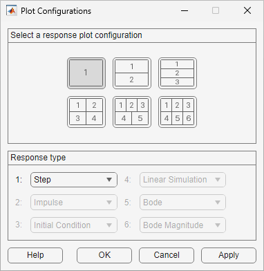
In the Select a response plot configuration section, select how many plots to show.
In the Response type section, use the drop-down lists to select the response type for each plot.
To update the plot configuration and close the dialog box, click OK.
To update the plot configuration without closing the dialog box, click Apply.
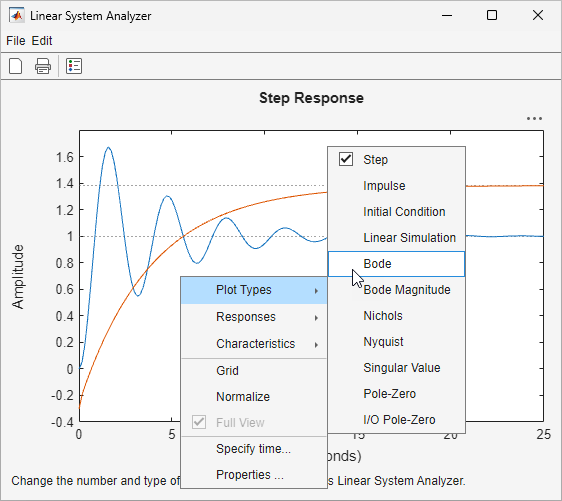
To switch the response type for an existing plot, right click the plot and, under Plot Types, select the type of response.
To interactively specify the line styles for responses, in Linear System Analyzer, select Edit > Response Styles. The Response Styles dialog box opens.
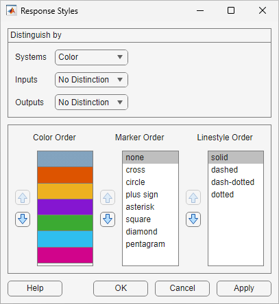
In the Distinguish by section, you can select how to distinguish between system, inputs, and outputs using the corresponding drop-down lists.
The selections in these drop-down lists are mutually exclusive, that is, you must use a different type of ordering for systems, inputs, and outputs.
Linear System Analyzer assigns response color, marker style, and line style based on the order specified under Color Order, Marker Order, and Linestyle Order, respectively.
You can modify these orders by clicking an item in the list and adjusting its position using the corresponding arrows.
To update the response styles and close the dialog box, click OK.
To update the response styles without closing the dialog box, click Apply.
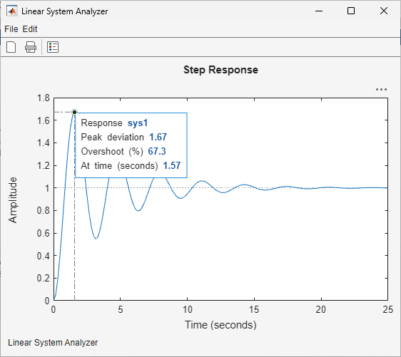
To display response characteristics in a response plot, right-click the plot area and, under Characteristics, select a characteristic to display. You can display multiple characteristics on the same plot.
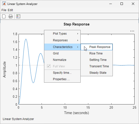
The available characteristics depend on the type of response plot.
| Response Plot | Available Characteristics |
|---|---|
| Step plot |
|
| Impulse plot |
|
| Initial condition plot | |
| Linear simulation plot | Peak response |
| Singular-value plot | |
| Bode plot |
|
| Nyquist plot | |
| Nichols plot | |
| Pole-zero plot | None |
| Pole/zero plot of each input/output pair |
The plot shows each characteristic using a marker on the response. To view information about the characteristic, click the marker.
Related Examples
Programmatic Use
Version History
Introduced in R2015a
See Also
Apps
Functions
stepplot|impulseplot|lsimplot|initialplot|iopzplot|pzplot|bodeplot|bodemag|nyquistplot|nicholsplot|sigmaplot