이 번역 페이지는 최신 내용을 담고 있지 않습니다. 최신 내용을 영문으로 보려면 여기를 클릭하십시오.
stepplot
계단 응답 플로팅 및 플롯 핸들 반환
구문
h = stepplot(sys)

stepplot(sys,Tfinal)

stepplot(sys,t)

stepplot(sys1,sys2,...,sysN)

stepplot(sys1,sys2,...,sysN,Tfinal)

stepplot(sys1,sys2,...,sysN,t)

stepplot(AX,...)

stepplot(..., plotoptions)

stepplot(..., dataoptions)
설명
h = stepplot(sys)는 동적 시스템 모델 sys의 계단 응답을 플로팅합니다. 또한 플롯 핸들 h도 반환합니다. getoptions 명령과 setoptions 명령에서 이 핸들을 사용하여 플롯을 사용자 지정할 수 있습니다. 다음을 입력합니다.
help timeoptions
사용 가능한 플롯 옵션을 볼 수 있습니다.
다중 입력 모델에서는 독립적인 계단 응답 명령이 각 입력 채널에 적용됩니다. 시간 범위와 점 개수는 자동으로 선택됩니다.
stepplot(sys,Tfinal)은 t = 0부터 최종 시간 t = Tfinal까지의 계단 응답을 시뮬레이션합니다. Tfinal을 sys의 TimeUnit 속성에 지정된 시스템 시간 단위로 표현합니다. 샘플 시간이 지정되지 않은(Ts = -1) 이산시간 시스템의 경우 stepplot은 Tfinal을 시뮬레이션할 샘플링 간격의 개수로 해석합니다.
stepplot(sys,t)는 시뮬레이션에 사용자가 제공한 시간 벡터 t를 사용합니다. t를 sys의 TimeUnit 속성에 지정된 시스템 시간 단위로 표현합니다. 이산시간 모델의 경우 t는 Ti:Ts:Tf 형식이어야 합니다. 여기서 Ts는 샘플 시간입니다. 연속시간 모델의 경우 t는 Ti:dt:Tf 형식이어야 합니다. 여기서 dt는 연속 시스템에 대한 이산 근사의 샘플 시간이 됩니다(step 참조). stepplot 명령은 Ti와 관계없이 항상 t=0에서 계단 입력을 적용합니다.
여러 모델 sys1,sys2,...의 계단 응답을 단일 플롯에 플로팅하려면 다음을 사용하십시오.
stepplot(sys1,sys2,...,sysN)
stepplot(sys1,sys2,...,sysN,Tfinal)
stepplot(sys1,sys2,...,sysN,t)
다음과 같이 각 시스템에 대해 색, 선 스타일 및 마커를 지정할 수도 있습니다.
stepplot(sys1,'r',sys2,'y--',sys3,'gx')
stepplot(AX,...)는 핸들 AX를 사용하여 좌표축에 플로팅합니다.
stepplot(..., plotoptions)는 옵션 세트 plotoptions를 사용하여 플롯 모양을 사용자 지정합니다. 옵션 세트를 만들려면 timeoptions를 사용하십시오.
stepplot(..., dataoptions)는 옵션 세트 dataoptions를 사용하여 계단 진폭, 입력 오프셋 같은 옵션을 지정합니다. 옵션 세트를 만들려면 stepDataOptions를 사용하십시오.
예제
두 동적 시스템에 대한 계단 응답 플롯을 생성합니다.
sys1 = rss(3);
sys2 = rss(3);
h = stepplot(sys1,sys2);

각 계단 응답은 서로 다른 정상 상태 값에 정착됩니다. 플로팅된 응답을 플롯 핸들을 사용하여 정규화합니다.
setoptions(h,'Normalize','on')
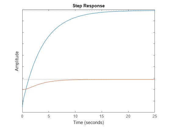
이제 응답은 임의 단위로 표현된 동일한 값에 정착됩니다.
식별된 모수적 모델의 계단 응답을 비모수적(경험적) 모델과 비교하고, 3-σ 신뢰영역을 확인합니다. 식별된 모델에는 System Identification Toolbox™가 필요합니다.
샘플 데이터에서 모수적 모델과 비모수적 모델을 식별합니다.
load iddata1 z1
sys1 = ssest(z1,4);
sys2 = impulseest(z1);
식별된 두 모델의 계단 응답을 플로팅합니다. 플롯 핸들을 사용하여 3-σ 신뢰영역을 표시합니다.
t = -1:0.1:5;
h = stepplot(sys1,sys2,t);
showConfidence(h,3)
legend('parametric','nonparametric')

비모수적 모델 sys2에서 불확실성이 더 높습니다.
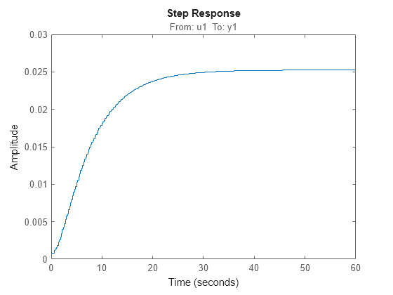
비선형 Hammerstein-Wiener 모델을 추정하기 위한 데이터를 불러옵니다.
load(fullfile(matlabroot,'toolbox','ident','iddemos','data','twotankdata'));
z = iddata(y,u,0.2,'Name','Two tank system');
z는 입력-출력 추정 데이터를 저장하는 iddata 객체입니다.
추정 데이터를 사용하여 차수가 [1 5 3]인 Hammerstein-Wiener 모델을 추정합니다. 입력 비선형성을 조각별 선형으로, 출력 비선형성을 1차원 다항식으로 지정합니다.
sys = nlhw(z,[1 5 3],pwlinear,poly1d);
입력 오프셋과 계단 진폭 수준을 지정하는 옵션 세트를 만듭니다.
opt = stepDataOptions('InputOffset',2,'StepAmplitude',0.5);
지정된 옵션을 사용하여 60초까지의 계단 응답을 플로팅합니다.
stepplot(sys,60,opt);
팁
한 예로 단위 같은 플롯의 속성을 변경할 수 있습니다. 플롯의 속성을 변경하는 방법에 대한 자세한 내용은 항목을 참조하십시오.
버전 내역
R2006a 이전에 개발됨
참고 항목
getoptions | setoptions | step