Modulation Classification by Using FPGA
This example shows how to deploy a pretrained convolutional neural network (CNN) for modulation classification to the Xilinx™ Zynq® UltraScale+™ MPSoC ZCU102 Evaluation Kit. The pretrained network is trained by using generated synthetic, channel-impaired waveforms.
Prerequisites
Xilinx™ Zynq® UltraScale+™ MPSoC ZCU102 Evaluation Kit
Predict Modulation Type by Using CNN
The trained CNN in this example recognizes these eight digital and three analog modulation types:
Binary phase shift keying (BPSK)
Quadrature phase shift keying (QPSK)
8-ary phase shift keying (8-PSK)
16-ary quadrature amplitude modulation (16-QAM)
64-ary quadrature amplitude modulation (64-QAM)
4-ary pulse amplitude modulation (PAM4)
Gaussian frequency shift keying (GFSK)
Continuous phase frequency shift keying (CPFSK)
Broadcast FM (B-FM)
Double sideband amplitude modulation (DSB-AM)
Single sideband amplitude modulation (SSB-AM)
modulationTypes = categorical(["BPSK", "QPSK", "8PSK", ...
  "16QAM", "64QAM", "PAM4", "GFSK", "CPFSK", ...
  "B-FM", "DSB-AM", "SSB-AM"]);
Load the trained network.
load dlhdltrainedModulationClassificationNetwork
trainedNet
trainedNet =
dlnetwork with properties:
Layers: [27×1 nnet.cnn.layer.Layer]
Connections: [26×2 table]
Learnables: [26×3 table]
State: [12×3 table]
InputNames: {'Input Layer'}
OutputNames: {'SoftMax'}
Initialized: 1
View summary with summary.
The trained CNN takes 1024 channel-impaired samples and predicts the modulation type of each frame. Generate several PAM4 frames that have Rician multipath fading, center frequency and sampling time drift, and AWGN. To generate synthetic signals to test the CNN, use the following functions. Then use the CNN to predict the modulation type of the frames.
randi: Generate random bitspammod(Communications Toolbox) PAM4-modulate the bitsrcosdesign(Signal Processing Toolbox): Design a square-root raised cosine pulse shaping filterfilter: Pulse shape the symbolscomm.RicianChannel(Communications Toolbox): Apply Rician multipath channelcomm.PhaseFrequencyOffset(Communications Toolbox): Apply phase and frequency shift due to clock offsetinterp1: Apply timing drift due to clock offsetawgn(Communications Toolbox): Add AWGN
% Set the random number generator to a known state to be able to regenerate
% the same frames every time the simulation is run
rng(123456)
% Random bits
d = randi([0 3], 1024, 1);
% PAM4 modulation
syms = pammod(d,4);
% Square-root raised cosine filter
filterCoeffs = rcosdesign(0.35,4,8);
tx = filter(filterCoeffs,1,upsample(syms,8));

% Channel
SNR = 30;
maxOffset = 5;
fc = 902e6;
fs = 200e3;
multipathChannel = comm.RicianChannel(...
    'SampleRate', fs, ...
    'PathDelays', [0 1.8 3.4] / 200e3, ...
    'AveragePathGains', [0 -2 -10], ...
    'KFactor', 4, ...
    'MaximumDopplerShift', 4);

frequencyShifter = comm.PhaseFrequencyOffset(...
    'SampleRate', fs);

% Apply an independent multipath channel
reset(multipathChannel)
outMultipathChan = multipathChannel(tx);

% Determine clock offset factor
clockOffset = (rand() * 2*maxOffset) - maxOffset;
C = 1 + clockOffset / 1e6;

% Add frequency offset
frequencyShifter.FrequencyOffset = -(C-1)*fc;
outFreqShifter = frequencyShifter(outMultipathChan);

% Add sampling time drift
t = (0:length(tx)-1)' / fs;
newFs = fs * C;
tp = (0:length(tx)-1)' / newFs;
outTimeDrift = interp1(t, outFreqShifter, tp);

% Add noise
rx = awgn(outTimeDrift,SNR,0);

% Frame generation for classification
unknownFrames = dlhdlhelperModClassGetNNFrames(rx);

% Classification
score1 = predict(trainedNet,unknownFrames);
Return the classifier predictions, which are analogous to hard decisions. The network correctly identifies the frames as PAM4 frames. For details on the generation of the modulated signals, see the dlhdlhelperModClassGetModulator function.
The classifier also returns a vector of scores for each frame. The score corresponds to the probability that each frame has the predicted modulation type. Plot the scores.
dlhdlhelperModClassPlotScores(score1,modulationTypes)

Waveform Generation for Training
Generate 10,000 frames for each modulation type, where 80% of the frames are used for training, 10% are used for validation and 10% are used for testing. Use the training and validation frames during the network training phase. You obtain the final classification accuracy by using test frames. Each frame is 1024 samples long and has a sample rate of 200 kHz. For digital modulation types, eight samples represent a symbol. The network makes each decision based on single frames rather than on multiple consecutive frames (as in video). Assume a center frequency of 902 MHz and 100 MHz for the digital and analog modulation types, respectively.
numFramesPerModType = 10000;
percentTrainingSamples = 80;
percentValidationSamples = 10;
percentTestSamples = 10;

sps = 8;                % Samples per symbol
spf = 1024;             % Samples per frame
symbolsPerFrame = spf / sps;
fs = 200e3;             % Sample rate
fc = [902e6 100e6];     % Center frequencies
Create Channel Impairments
Pass each frame through a channel by using:
AWGN
Rician multipath fading
Clock offset, resulting in center frequency offset and sampling time drift
Because the network in this example makes decisions based on single frames, each frame must pass through an independent channel AWGN.
The channel adds AWGN by using an SNR of 30 dB. Implement the channel by using the awgn (Communications Toolbox) function.
Rician Multipath
The channel passes the signals through a Rician multipath fading channel by using the comm.RicianChannel (Communications Toolbox) System object. Assume a delay profile of [0 1.8 3.4] samples that have corresponding average path gains of [0 -2 -10] dB. The K-factor is 4 and the maximum Doppler shift is 4 Hz, which is equivalent to a walking speed at 902 MHz. Implement the channel by using the following settings.
Clock Offset
Clock offset occurs because of the inaccuracies of internal clock sources of transmitters and receivers. Clock offset causes the center frequency, which is used to downconvert the signal to baseband, and the digital-to-analog converter sampling rate to differ from theoretical values. The channel simulator uses the clock offset factor C, expressed as C=1+Δclock106, where Δclock is the clock offset. For each frame, the channel generates a random Δclock value from a uniformly distributed set of values in the range [−maxΔclock maxΔclock], where maxΔclock is the maximum clock offset. Clock offset is measured in parts per million (ppm). For this example, assume a maximum clock offset of 5 ppm.
maxDeltaOff = 5;
deltaOff = (rand()*2*maxDeltaOff) - maxDeltaOff;
C = 1 + (deltaOff/1e6);
Frequency Offset
Subject each frame to a frequency offset based on clock offset factor C and the center frequency. Implement the channel by using the comm.PhaseFrequencyOffset (Communications Toolbox).
Sampling Rate Offset
Subject each frame to a sampling rate offset based on clock offset factor C. Implement the channel by using the interp1 function to resample the frame at the new rate of C×fs.
Combined Channel
To apply all three channel impairments to the frames, use the dlhdlhelperModClassTestChannel object.
channel = dlhdlhelperModClassTestChannel(...
  'SampleRate', fs, ...
  'SNR', SNR, ...
  'PathDelays', [0 1.8 3.4] / fs, ...
  'AveragePathGains', [0 -2 -10], ...
  'KFactor', 4, ...
  'MaximumDopplerShift', 4, ...
  'MaximumClockOffset', 5, ...
  'CenterFrequency', 902e6)
channel =
  dlhdlhelperModClassTestChannel with properties:

                    SNR: 30
        CenterFrequency: 902000000
             SampleRate: 200000
             PathDelays: [0 9.0000e-06 1.7000e-05]
       AveragePathGains: [0 -2 -10]
                KFactor: 4
    MaximumDopplerShift: 4
     MaximumClockOffset: 5
You can view basic information about the channel by using the info object function.
chInfo = info(channel)
chInfo = struct with fields:
               ChannelDelay: 6
     MaximumFrequencyOffset: 4510
    MaximumSampleRateOffset: 1
Waveform Generation
Create a loop that generates channel-impaired frames for each modulation type and stores the frames with their corresponding labels in MAT files. By saving the data into files, you do not have to eliminate the need to generate the data every time you run this example. You can also share the data more effectively.
Remove a random number of samples from the beginning of each frame to remove transients and to make sure that the frames have a random starting point with respect to the symbol boundaries.
% Set the random number generator to a known state to be able to regenerate
% the same frames every time the simulation is run
rng(1235)
tic

numModulationTypes = length(modulationTypes);

channelInfo = info(channel);
transDelay = 50;
dataDirectory = fullfile(tempdir,"ModClassDataFiles");
disp("Data file directory is " + dataDirectory);
Data file directory is /tmp/ModClassDataFiles
fileNameRoot = "frame";

% Check if data files exist
dataFilesExist = false;
if exist(dataDirectory,'dir')
  files = dir(fullfile(dataDirectory,sprintf("%s*",fileNameRoot)));
  if length(files) == numModulationTypes*numFramesPerModType
    dataFilesExist = true;
  end
end

if ~dataFilesExist
  disp("Generating data and saving in data files...")
  [success,msg,msgID] = mkdir(dataDirectory);
  if ~success
    error(msgID,msg)
  end
  for modType = 1:numModulationTypes
    elapsedTime = seconds(toc);
    elapsedTime.Format = 'hh:mm:ss';
    fprintf('%s - Generating %s frames\n', ...
      elapsedTime, modulationTypes(modType))

    label = modulationTypes(modType);
    numSymbols = (numFramesPerModType / sps);
    dataSrc = dlhdlhelperModClassGetSource(modulationTypes(modType), sps, 2*spf, fs);
    modulator = dlhdlhelperModClassGetModulator(modulationTypes(modType), sps, fs);
    if contains(char(modulationTypes(modType)), {'B-FM','DSB-AM','SSB-AM'})
      % Analog modulation types use a center frequency of 100 MHz
      channel.CenterFrequency = 100e6;
    else
      % Digital modulation types use a center frequency of 902 MHz
      channel.CenterFrequency = 902e6;
    end

    for p=1:numFramesPerModType
      % Generate random data
      x = dataSrc();

      % Modulate
      y = modulator(x);

      % Pass through independent channels
      rxSamples = channel(y);

      % Remove transients from the beginning, trim to size, and normalize
      frame = dlhdlhelperModClassFrameGenerator(rxSamples, spf, spf, transDelay, sps);

      % Save data file
      fileName = fullfile(dataDirectory,...
        sprintf("%s%s%03d",fileNameRoot,modulationTypes(modType),p));
      save(fileName,"frame","label")
    end
  end
else
  disp("Data files exist. Skip data generation.")
end
Generating data and saving in data files...
00:00:13 - Generating BPSK frames
00:01:18 - Generating QPSK frames
00:02:26 - Generating 8PSK frames
00:03:28 - Generating 16QAM frames
00:04:32 - Generating 64QAM frames
00:05:36 - Generating PAM4 frames
00:06:36 - Generating GFSK frames
00:07:34 - Generating CPFSK frames
00:08:34 - Generating B-FM frames
00:10:06 - Generating DSB-AM frames
00:11:07 - Generating SSB-AM frames
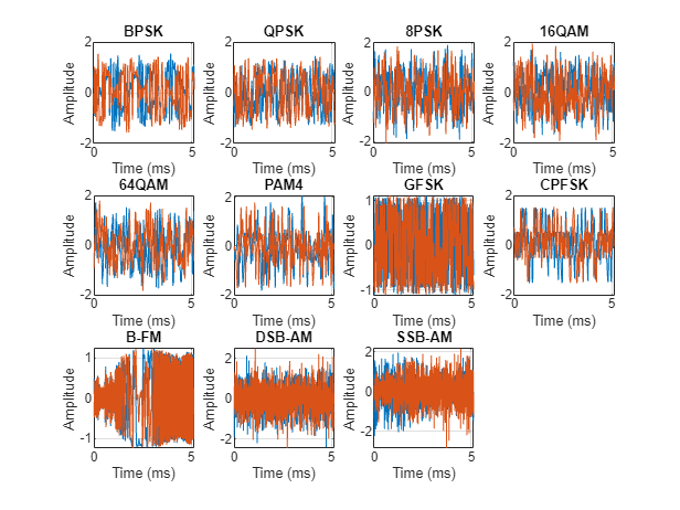
% Plot the amplitude of the real and imaginary parts of the example frames
% against the sample number
dlhdlhelperModClassPlotTimeDomain(dataDirectory,modulationTypes,fs)
% Plot the spectrogram of the example frames
dlhdlhelperModClassPlotSpectrogram(dataDirectory,modulationTypes,fs,sps)
Create a Datastore
To manage the files that contain the generated complex waveforms, use a signalDatastore object. Datastores are especially useful when each individual file fits in memory, but the entire collection does not necessarily fit.
frameDS = signalDatastore(dataDirectory,'SignalVariableNames',["frame","label"]);
Transform Complex Signals to Real Arrays
The deep learning network in this example looks for real inputs while the received signal has complex baseband samples. Transform the complex signals into real-valued 4-D arrays. The output frames have size 1-by-spf-by-2-by-N, where the first page (3rd dimension) is in-phase samples and the second page is quadrature samples. When the convolutional filters are of size 1-by-spf, this approach ensures that the information in the I and Q is mixed even in the convolutional layers and makes better use of the phase information. See dlhdlhelperModClassIQAPages.
frameDSTrans = transform(frameDS,@dlhdlhelperModClassIQAsPages);
Split into Training, Validation, and Test
Divide the frames into training, validation, and test data. See dlhdlhelperModClassSplitData.
splitPercentages = [percentTrainingSamples,percentValidationSamples,percentTestSamples];
[trainDSTrans,validDSTrans,testDSTrans] = dlhdlhelperModClassSplitData(frameDSTrans,splitPercentages);
Starting parallel pool (parpool) using the 'Processes' profile ...
Connected to parallel pool with 6 workers.
Import Data Into Memory
Neural network training is iterative. At every iteration, the datastore reads data from files and transforms the data before updating the network coefficients. If the data fits into the memory of your computer, importing the data from the files into the memory enables faster training by eliminating this repeated read from file and transform process. Instead, the data is read from the files and transformed once. Training this network using data files on disk takes about 110 minutes while training using in-memory data takes about 50 minutes.
Import the data in the files into memory. The files have two variables: frame and label. Each read call to the datastore returns a cell array, where the first element is the frame and the second element is the label. To read frames and labels, use the transform functions dlhdlhelperModClassReadFrame and dlhdlhelperModClassReadLabel. Use readall with the "UseParallel" option set to true to enable parallel processing of the transform functions, if you have Parallel Computing Toolbox license. Because the readall function, by default, concatenates the output of the read function over the first dimension, return the frames in a cell array and manually concatenate over the fourth dimension.
% Read the training and validation frames into the memory
pctExists = parallelComputingLicenseExists();
trainFrames = transform(trainDSTrans, @dlhdlhelperModClassReadFrame);
rxTrainFrames = readall(trainFrames,"UseParallel",pctExists);
rxTrainFrames = cat(4, rxTrainFrames{:});
validFrames = transform(validDSTrans, @dlhdlhelperModClassReadFrame);
rxValidFrames = readall(validFrames,"UseParallel",pctExists);
rxValidFrames = cat(4, rxValidFrames{:});

% Read the training and validation labels into the memory
trainLabels = transform(trainDSTrans, @dlhdlhelperModClassReadLabel);
rxTrainLabels = readall(trainLabels,"UseParallel",pctExists);
validLabels = transform(validDSTrans, @dlhdlhelperModClassReadLabel);
rxValidLabels = readall(validLabels,"UseParallel",pctExists);
testFrames = transform(testDSTrans, @dlhdlhelperModClassReadFrame);
rxTestFrames = readall(testFrames,"UseParallel",pctExists);
rxTestFrames = cat(4, rxTestFrames{:});

% Read the test labels into the memory
YPred = transform(testDSTrans, @dlhdlhelperModClassReadLabel);
rxTestLabels = readall(YPred,"UseParallel",pctExists);
Create Target Object
Create a target object for your target device that has a vendor name and an interface to connect your target device to the host computer. Interface options are JTAG (default) and Ethernet. Vendor options are Intel or Xilinx. To program the device, use the installed Xilinx Vivado Design Suite over an Ethernet connection.
hT = dlhdl.Target('Xilinx', Interface = 'Ethernet');
Create Workflow Object
Create an object of the dlhdl.Workflow class. When you create the object, specify the network and the bitstream name. Specify the saved pretrained dlnetwork trainedAudioNet as the network. Make sure that the bitstream name matches the data type and the FPGA board that you are targeting. In this example, the target FPGA board is the Zynq UltraScale+ MPSoC ZCU102 board. The bitstream uses a single data type.
hW = dlhdl.Workflow(Network = trainedNet, Bitstream = 'zcu102_single', Target = hT);Compile trainedModulationClassification Network
To compile the trainedNet dlnetwork, run the compile function of the dlhdl.Workflow object.
compile(hW)
### Compiling network for Deep Learning FPGA prototyping ...
### Targeting FPGA bitstream zcu102_single.
### An output layer called 'Output1_SoftMax' of type 'nnet.cnn.layer.RegressionOutputLayer' has been added to the provided network. This layer performs no operation during prediction and thus does not affect the output of the network.
### Optimizing network: Fused 'nnet.cnn.layer.BatchNormalizationLayer' into 'nnet.cnn.layer.Convolution2DLayer'
### Optimizing network: Non-symmetric stride of layer with name 'MaxPool1' made symmetric as it produces an equivalent result, and only symmetric strides are supported.
### Optimizing network: Non-symmetric stride of layer with name 'MaxPool2' made symmetric as it produces an equivalent result, and only symmetric strides are supported.
### Optimizing network: Non-symmetric stride of layer with name 'MaxPool3' made symmetric as it produces an equivalent result, and only symmetric strides are supported.
### Optimizing network: Non-symmetric stride of layer with name 'MaxPool4' made symmetric as it produces an equivalent result, and only symmetric strides are supported.
### Optimizing network: Non-symmetric stride of layer with name 'MaxPool5' made symmetric as it produces an equivalent result, and only symmetric strides are supported.
### The network includes the following layers:

### Notice: The layer 'Input Layer' with type 'nnet.cnn.layer.ImageInputLayer' is implemented in software.
### Notice: The layer 'SoftMax' with type 'nnet.cnn.layer.SoftmaxLayer' is implemented in software.
### Notice: The layer 'Output1_SoftMax' with type 'nnet.cnn.layer.RegressionOutputLayer' is implemented in software.
### Compiling layer group: CNN1>>ReLU6 ...
### Compiling layer group: CNN1>>ReLU6 ... complete.
### Compiling layer group: AP1 ...
### Compiling layer group: AP1 ... complete.
### Compiling layer group: FC1 ...
### Compiling layer group: FC1 ... complete.

### Allocating external memory buffers:

          offset_name          offset_address     allocated_space
    _______________________    ______________    __________________

    "InputDataOffset"           "0x00000000"     "480.0 kB"
    "OutputResultOffset"        "0x00078000"     "4.0 kB"
    "SchedulerDataOffset"       "0x00079000"     "32.0 kB"
    "SystemBufferOffset"        "0x00081000"     "148.0 kB"
    "InstructionDataOffset"     "0x000a6000"     "72.0 kB"
    "ConvWeightDataOffset"      "0x000b8000"     "1.9 MB"
    "FCWeightDataOffset"        "0x0029b000"     "8.0 kB"
    "EndOffset"                 "0x0029d000"     "Total: 2676.0 kB"

### Network compilation complete.
ans = struct with fields:
             weights: [1×1 struct]
        instructions: [1×1 struct]
           registers: [1×1 struct]
    syncInstructions: [1×1 struct]
        constantData: {}
             ddrInfo: [1×1 struct]
       resourceTable: [6×2 table]
Program Bitstream onto FPGA and Download Network Weights
To deploy the network on the Zynq® UltraScale+™ MPSoC ZCU102 hardware, run the deploy function of the dlhdl.Workflow object. This function uses the output of the compile function to program the FPGA board by using the programming file.The function also downloads the network weights and biases. The deploy function verifies the Xilinx Vivado tool and the supported tool version. It then starts programming the FPGA device by using the bitstream, displays progress messages, and the time it takes to deploy the network.
deploy(hW)
### Programming FPGA Bitstream using Ethernet...
### Attempting to connect to the hardware board at 172.21.88.150...
### Connection successful
### Programming FPGA device on Xilinx SoC hardware board at 172.21.88.150...
### Attempting to connect to the hardware board at 172.21.88.150...
### Connection successful
### Copying FPGA programming files to SD card...
### Setting FPGA bitstream and devicetree for boot...
# Copying Bitstream zcu102_single.bit to /mnt/hdlcoder_rd
# Set Bitstream to hdlcoder_rd/zcu102_single.bit
# Copying Devicetree devicetree_dlhdl.dtb to /mnt/hdlcoder_rd
# Set Devicetree to hdlcoder_rd/devicetree_dlhdl.dtb
# Set up boot for Reference Design: 'AXI-Stream DDR Memory Access : 3-AXIM'
### Programming done. The system will now reboot for persistent changes to take effect.
### Rebooting Xilinx SoC at 172.21.88.150...
### Reboot may take several seconds...
### Attempting to connect to the hardware board at 172.21.88.150...
### Connection successful
### Programming the FPGA bitstream has been completed successfully.
### Loading weights to Conv Processor.
### Conv Weights loaded. Current time is 29-Aug-2024 08:51:58
### Loading weights to FC Processor.
### FC Weights loaded. Current time is 29-Aug-2024 08:51:59
Results
Classify five inputs from the test data set and compare the prediction results to the classification results from the Deep Learning Toolbox™. The YPred variable is the classification results from the Deep learning Toolbox™. The fpga_prediction variable is the classification result from the FPGA.
numtestFrames = size(rxTestFrames,4);
numView = 5;
listIndex = randperm(numtestFrames,numView);
testDataBatch = rxTestFrames(:,:,:,listIndex);
testDataBatch = dlarray(testDataBatch, 'SSCB');
YPred = predict(trainedNet,testDataBatch);
[scores,speed] = predict(hW,testDataBatch, Profile ='on');
### Finished writing input activations.
### Running in multi-frame mode with 5 inputs.


              Deep Learning Processor Profiler Performance Results

                   LastFrameLatency(cycles)   LastFrameLatency(seconds)       FramesNum      Total Latency     Frames/s
                         -------------             -------------              ---------        ---------       ---------
Network                     675167                  0.00307                       5            3368758            326.5
    CNN1                     30145                  0.00014
    MaxPool1                 15512                  0.00007
    CNN2                     68492                  0.00031
    MaxPool2                 11627                  0.00005
    CNN3                     84161                  0.00038
    MaxPool3                  8599                  0.00004
    CNN4                    119791                  0.00054
    MaxPool4                  7232                  0.00003
    CNN5                    155982                  0.00071
    MaxPool5                  5059                  0.00002
    CNN6                    155066                  0.00070
    AP1                      11956                  0.00005
    FC1                       1499                  0.00001
 * The clock frequency of the DL processor is: 220MHz
YPred = scores2label(YPred,categories(modulationTypes));
fpga_prediction = scores2label(scores,categories(modulationTypes));
Compare the prediction results from Deep Learning Toolbox™ and the FPGA side by side. The prediction results from the FPGA match the prediction results from Deep Learning Toolbox™. In this table, the ground truth prediction is the Deep Learning Toolbox™ prediction.
fprintf('%12s %24s\n','Ground Truth','FPGA Prediction');for i= 1:size(fpga_prediction,2)
fprintf('%s %24s\n',YPred(i),fpga_prediction(i)); end
Ground Truth FPGA Prediction
16QAM                    16QAM
GFSK                     GFSK
64QAM                    64QAM
CPFSK                    CPFSK
B-FM                     B-FM
References
O'Shea, T. J., J. Corgan, and T. C. Clancy. "Convolutional Radio Modulation Recognition Networks." Preprint, submitted June 10, 2016. https://arxiv.org/abs/1602.04105
O'Shea, T. J., T. Roy, and T. C. Clancy. "Over-the-Air Deep Learning Based Radio Signal Classification." IEEE Journal of Selected Topics in Signal Processing. Vol. 12, Number 1, 2018, pp. 168–179.
Liu, X., D. Yang, and A. E. Gamal. "Deep Neural Network Architectures for Modulation Classification." Preprint, submitted January 5, 2018. https://arxiv.org/abs/1712.00443v3
See Also
Topics
- Modulation Classification with Deep Learning
- Deep Learning in MATLAB (Deep Learning Toolbox)