Phase and gain margins
From the series: Using Bode Plots
Learn what gain margin and phase margins are and how to use them for control design in this MATLAB® Tech Talk by Carlos Osorio.
Published: 29 Apr 2013
In order to better understand what is going on around the crossover frequency point, let us first talk briefly about the stability of our closed loop system. In general, for any feedback control architecture, all the relevant closed loop transfer functions will have the same characteristic polynomial in the denominator, and the stability of the system will be determined by the roots of that polynomial.
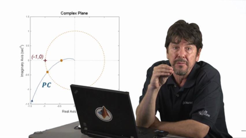
In our case, that characteristic polynomial is 1+PC. In terms of the frequency response, this expression will be zero if and only if the open loop transfer function PC happens to be equal to -1 -- I mean, real -1, or (-1, 0) on a complex plane. Remember that when we replace errors by jw, the product of the transfer function P and C becomes a complex vector that will have a magnitude and a phase that are functions of w.
This plot, by the way, is called a Nyquist diagram, and notice that it is constructed with the same information we use for the Bode diagram. The main difference is that, whereas the Bode plot displays the magnitude and the phase of your transfer function in two separate axes, the Nyquist plot displays both quantities in a single plot on a real versus imaginary plane. For each different value of w, the magnitude and the phase of that vector will give us a unique point on the diagram. And if we sweep for all values of w going from 0 to infinity, we will end up with a complete frequency response trace for our transfer function.
In this case, we are looking at Nyquist plot of our open loop transfer function PC. Notice that if the trace of PC were to pass through the (-1, 0) point, then at that point for that excitation frequency, the denominator of our closed loop transfer function would become 0, which means that both T and S will go to infinity, and obviously, our system will blow up, which, as you might guess, would be really bad. So that (-1, 0) is that critical stability boundary, and we want to make sure that our open loop design, whatever it is, stays far enough away from it. The question is, how far away?
Just as a quick aside, we know that determining the stability of our closed loop system means finding the roots of 1+PC are stable, meaning they are all on the left-hand side of the complex plane. Depending on the order of the numerator and denominator of our controller and plant, the resulting characteristic polynomial can be a bit cumbersome to solve by inspection. So that's why we use things like Routh-Hurwitz, which determines if the roots of a polynomial will be positive or negative just by looking at its coefficients, or the Nyquist criterion, which determines that closed loop system stability by relating the number of zeros and poles on your open loop transfer function to the number of times the frequency tracing, the Nyquist diagram, encircles that (-1, 0) point.
Anyways, I don't want to overcomplicate this. So let me just assume that we have a simple stable system. As I was saying before, the real question becomes, how stable is it? To answer this, we will look at two critical points on our open loop trace, one where the magnitude of our trace is equal to 1, and the other where the phase angle of our trace is equal to -180 degrees.
We obviously do not want both of this to be the same because that will mean that we are on top of that (-1,0) point. So, the stability margins we are looking for are akin to defining a safety region that ensures we are far enough away from that point.
In simple terms, the angle safety factor, or phase margin, indicates how much extra phase lag we can have before becoming unstable. And the magnitude safety factor, or gain margin, indicates how much additional gain we can have before becoming unstable.
If I may use an analogy to help me explain both these numbers, think of a downhill skier on a slalom course. To maximize his speed, he will have made in his head a plan for an ideal or desired path that will take him through those gates in some sort of optimized fashion. When he goes down the course, his actual path may lag a little bit from the desired path, but still he might be able to make it all the way to the finish line. But if his actual turns start lagging too far behind his ideal path, there will be a point where that lag becomes too much, and he won't be able to recover, and more than likely will end up crashing or missing a gate. In other words, he violated his phase margin. Similarly, with the gain margin, think of the system gain as how hard or sharp the skier makes his turns. If his turning motion is too sharp, meaning he's using too much gain, he will end up overcorrecting and overshooting to one side of the desired path, and then back to the other, losing the course and eventually crashing somewhere.
Anyways, coming back to our Bode diagram, the (-1, 0) point will be worth that magnitude is 1, which means 0 dBs on the plot, and the phase is -180 degrees. Just think of 180 degrees lag as our controller pushing when it should be pulling, or vice versa, the skier turning right when he should be turning left. Not much good can come out of that.
The phase margin is measured as the difference between the phase trace and the -180 degrees line at the frequency where the magnitude crosses 0 dBs. For stability, we need the phase margin to be greater than 0, but usually we will want to keep it above 45 degrees. A phase margin of 60 degrees is usually recommended for a relatively smooth, well damped system behavior.
The gain margin is measured as the reciprocal of the magnitude at the point where the phase crosses -180 degrees. The reciprocal in a logarithmic scale means a sign change. So for stability, the gain margin needs to be a positive value. Anywhere above 5 dBs is usually recommended.
So just to summarize, one of the key values of the stability margins is that they not only allow us to determine the overall stability of our closed loop system directly from our open loop design, but they also give us a sense for how stable we are. Good stability margins, to a point, of course, can guarantee a certain level of performance and can protect us from uncertainties and unmodeled perturbations in our system dynamics.


