다음에 대한 결과:
The Cody Contest 2025 is underway, and it includes a super creative problem group which many of us have found fascinating. The central theme of the problems, expertly curated by @Matt Tearle, humorously revolves around the whims of the capricious dictator Lord Ned, as he goes out of his way to complicate the lives of his subjects and visitors alike. We cannot judge whether or not there's any truth to the rumors behind all the inside jokes, but it's obvious that the team had a lot of fun creating these; and we had even more fun solving them.
Today I want to showcase a way of graphically solving and visualizing one of those problems which I found very elegant, The Bridges of Nedsburg.
To briefly reiterate the problem, the number of islands and the arrangement of bridges of the city of Nedsburg are constantly changing. Lord Ned has decided to take advantage of this by charging visitors with an increasingly expensive n-bridge pass which allows them to cross up to n bridges in one journey. Given the Connectivity Matrix C, we are tasked with calculating the minimum n needed so that there is a path from every island to every other island in n steps or fewer.
Matt kindly provided us with some useful bit of math in the description detailing how to calculate the way to get from one island to another in an number of m steps. However, he has also hidden an alternative path to the solution in plain sight, in one of the graphs he provided. This involves the extremely useful and versatile object digraph, representing directed graphs, which have directional edges connecting the nodes. Here's some further great documentation and other cool resources on the topic for those who are interested in learning more about it:
Let's start using this object to explore a graphical solution to Lord Ned's conundrum. We will use the unit tests included in the problem to visualize the solution. We can retrieve the connectivity matrix for each case using the following function:
function C = getConnectivityMatrix(unit_test)
% Number of islands and bridge arrangement
switch unit_test
case 1
m = 3; idx = [3;4;8];
case 2
m = 3; idx = [3;4;7;8];
case 3
m = 4; idx = [2;7;8;10;13];
case 4
m = 4; idx = [4;5;7;8;9;14];
case 5
m = 5; idx = [5;8;11;12;14;18;22;23];
case 6
m = 5; idx = [2;5;8;14;20;21;24];
case 7
m = 6; idx = [3;4;7;11;18;23;24;26;30;32];
case 8
m = 6; idx = [3;11;12;13;18;19;28;32];
case 9
m = 7; idx = [3;4;6;8;13;14;20;21;23;31;36;47];
case 10
m = 7; idx = [4;11;13;14;19;22;23;26;28;30;34;35;37;38;45];
case 11
m = 8; idx = [2;4;5;6;8;12;13;17;27;39;44;48;54;58;60;62];
case 12
m = 8; idx = [3;9;12;20;24;29;30;31;33;44;48;50;53;54;58];
case 13
m = 9; idx = [8;9;10;14;15;22;25;26;29;33;36;42;44;47;48;50;53;54;55;67;80];
case 14
m = 9; idx = [8;10;22;32;37;40;43;45;47;53;56;57;62;64;69;70;73;77;79];
case 15
m = 10; idx = [2;5;8;13;16;20;24;27;28;36;43;49;53;62;71;75;77;83;86;87;95];
case 16
m = 10; idx = [4;9;14;21;22;35;37;38;44;47;50;51;53;55;59;61;63;66;69;76;77;84;85;86;90;97];
end
C = zeros(m);
C(idx) = 1;
end
The case in the example refers to unit test case 2.
unit_test = 2;
C = getConnectivityMatrix(unit_test);
disp(C)
D = digraph(C);
figure
p = plot(D,'LineWidth',1.5,'ArrowSize',10);
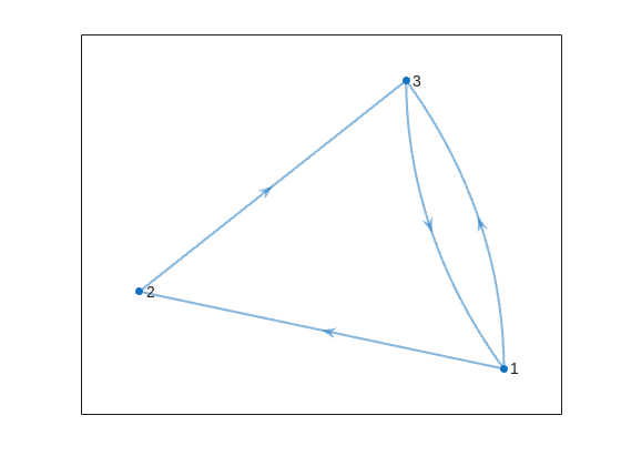
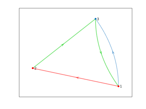
This is the same as the graph provided in the example. Another very useful method of digraph is shortestpath. This allows us to calculate the path and distance from one single node to another. For example:
% Path and distance from node 1 to node 2
[path12,dist12] = shortestpath(D,1,2);
fprintf('The shortest path from island %d to island %d is: %s. The minimum number of steps is: n = %d\n', 1, 2, join(string(path12), ' -> '),dist12)
% Path and distance from node 2 to node 1
[path21,dist21] = shortestpath(D,2,1);
fprintf('The shortest path from island %d to island %d is: %s. The minimum number of steps is: n = %d\n', 2, 1, join(string(path21), ' -> '),dist21)
figure
p = plot(D,'LineWidth',1.5,'ArrowSize',10);
highlight(p,path12,'EdgeColor','r','NodeColor','r','LineWidth',2)
highlight(p,path21,'EdgeColor',[0 0.8 0],'LineWidth',2)
But that's not all! digraph can also provide us with a matrix of the distances d, i.e. the steps needed to travel from island i to island j, where i and j are the rows and columns of d respectively. This is accomplished by using its distances method. The distance matrix can be visualized as:
d = distances(D);
figure
% Using pcolor w/ appending matrix workaround for convenience
pcolor([d,d(:,end);d(end,:),d(end,end)])
% Alternatively you can use imagesc(d), but you'll have to recreate the grid manually
axis square
set(gca,'YDir','reverse','XTick',[],'YTick',[])
[X,Y] = meshgrid(1:height(d));
text(X(:)+0.5,Y(:)+0.5,string(d(:)),'FontSize',11)
colormap(interp1(linspace(0,1,4), [1 1 1; 0.7 0.9 1; 0.6 0.7 1; 1 0.3 0.3], linspace(0,1,8)))
clim([-0.5 7+0.5])
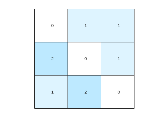
This confirms what we saw before, i.e. you need 1 step to go from island 1 to island 2, but 2 steps for vice versa. It also confirms that the minimum number of steps n that you need to buy the pass for is 2 (which also occurs for traveling from island 3 to island 2). As it's not the point of the post to give the full solution to the problem but rather present the graphical way of visualizing it I will not include the code of how to calculate this, but I'm sure that by now it's reduced to a trivial problem which you have already figured out how to solve.
That being said, now that we have the distance matrix, let's continue with the visualizations. First, let's plot the corresponding paths for each of these combinations:
figure
tiledlayout(size(C,1),size(C,2),'TileSpacing','tight','Padding','tight');
for i = 1:size(C,1)
for j = 1:size(C,2)
nexttile
p = plot(D,'ArrowSize',10);
highlight(p,shortestpath(D,i,j),'EdgeColor','r','NodeColor','r','LineWidth',2)
lims = axis;
text(lims(1)+diff(lims(1:2))*0.05,lims(3)+diff(lims(3:4))*0.9,sprintf('n = %d',d(i,j)))
end
end
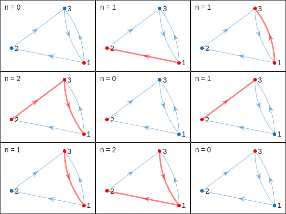
This allows us to go from the distance matrix to visualizing the paths and number of steps for each corresponding case. Things are rather simple for this 3-island example case, but evil Lord Ned is just getting started. Let's now try to solve the problem for all provided unit test cases:
% Cell array of connectivity matrices
C = arrayfun(@getConnectivityMatrix,1:16,'UniformOutput',false);
% Cell array of corresponding digraph objects
D = cellfun(@digraph,C,'UniformOutput',false);
% Cell array of corresponding distance matrices
d = cellfun(@distances,D,'UniformOutput',false);
% id of solutions: Provided as is to avoid handing out the code to the full solution
id = [2, 2, 9, 3, 4, 6, 16, 4, 44, 43, 33, 34, 7, 18, 39, 2];
First, let's plot the distance matrix for each case:
figure
tiledlayout('flow','TileSpacing','compact','Padding','compact');
% Vary this to plot different combinations of cases
plot_cases = 1:numel(C);
for i = plot_cases
nexttile
pcolor([d{i},d{i}(:,end);d{i}(end,:),d{i}(end,end)])
axis square
set(gca,'YDir','reverse','XTick',[],'YTick',[])
title(sprintf('Case %d',i),'FontWeight','normal','FontSize',8)
end
c = colorbar('Ticks',0:7,'TickLength',0,'Limits',[-0.5 7+0.5],'FontSize',8);
c.Layout.Tile = 'East';
c.Label.String = 'Number of Steps';
c.Label.FontSize = 8;
colormap(interp1(linspace(0,1,4), [1 1 1; 0.7 0.9 1; 0.6 0.7 1; 1 0.3 0.3], linspace(0,1,8)))
clim(findobj(gcf,'type','axes'),[-0.5 7+0.5])
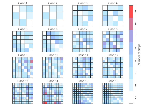
We immediately notice some inconsistencies, perhaps to be expected of the eccentric and cunning dictator. Things are pretty simple for the configurations with a small number of islands, but the minimum number of steps n can increase sharply and disproportionally to the additional number of islands. Cases 8 and 9 in particular have a particularly large n (relative to their grid dimensions), and case 14 has the largest n, almost double that of case 16 despite the fact that the latter has one extra island.
To visualize how this is possible, let's plot the path corresponding to the largest n for each case (though note that there might be multiple possible paths for each case):
figure
tiledlayout('flow','TileSpacing','tight','Padding','tight');
for i = plot_cases
nexttile
% Changing the layout to circular so we can better visualize the paths
p = plot(D{i},'ArrowSize',10,'Layout','Circle');
% Alternatively we could use the XData and YData properties if the positions of the islands were provided
axis([-1.5 1.5 -1.5 1.75])
[row,col] = ind2sub(size(d{i}),id(i));
highlight(p,shortestpath(D{i},row,col),'EdgeColor','r','NodeColor','r','LineWidth',2)
lims = axis;
text(lims(1)+diff(lims(1:2))*0.05,lims(3)+diff(lims(3:4))*0.9,sprintf('n = %d',d{i}(row,col)))
end
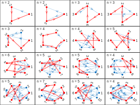
And busted! Unraveled! Exposed! Lord Ned has clearly been taking advantages of the tectonic forces by instructing his corrupt civil engineer lackeys to design the bridges to purposely force the visitors to go around in circles in order to drain them of their precious savings. In particular, for cases 8 and 9, he would have them go through every single island just to get from one island to another, whereas for case 14 they would have to visit 8 of the 9 islands just to get to their destination. If that's not diabolical then I don't know what is!
Ned jokes aside, I hope you enjoyed this contest just as much as I did, and that you found this article useful. I look forward to seeing more creative problems and solutions in the future.
Trinity
- It's the question that drives us, Neo. It's the question that brought you here. You know the question, just as I did.
Neo
- What is the Matlab?
Morpheus
- Unfortunately, no one can be told what the Matlab is. You have to see it for yourself.
And also later :
Morpheus
- The Matlab is everywhere. It is all around us. Even now, in this very room. You can feel it when you go to work [...]
The Architect
- The first Matlab I designed was quite naturally perfect. It was a work of art. Flawless. Sublime.
[My Matlab quotes version of the movie (Matrix, 1999) ]
2 x 2 행렬의 행렬식은
- 행렬의 두 row 벡터로 정의되는 평행사변형의 면적입니다.
- 물론 두 column 벡터로 정의되는 평행사변형의 면적이기도 합니다.
- 좀 더 정확히는 signed area입니다. 면적이 음수가 될 수도 있다는 뜻이죠.
- 행렬의 두 행(또는 두 열)을 맞바꾸면 행렬식의 부호도 바뀌고 면적의 부호도 바뀌어야합니다.
일반적으로 n x n 행렬의 행렬식은
- 각 row 벡터(또는 각 column 벡터)로 정의되는 N차원 공간의 평행면체(?)의 signed area입니다.
- 제대로 이해하려면 대수학의 개념을 많이 가지고 와야 하는데 자세한 설명은 생략합니다.(=저도 모른다는 뜻)
- 더 자세히 알고 싶으시면 수학하는 만화의 '넓이 이야기' 편을 추천합니다.
- 수학적인 정의를 알고 싶으시면 위키피디아를 보시면 됩니다.
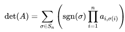
- 이렇게 생겼습니다. 좀 무섭습니다.
아래 코드는...
- 2 x 2 행렬에 대해서 이것을 수식 없이 그림만으로 증명하는 과정입니다.
- gif 생성에는 ScreenToGif를 사용했습니다. (gif 만들기엔 이게 킹왕짱인듯)
Determinant of 2 x 2 matrix is...
- An area of a parallelogram defined by two row vectors.
- Of course, same one defined by two column vectors.
- Precisely, a signed area, which means area can be negative.
- If two rows (or columns) are swapped, both the sign of determinant and area change.
More generally, determinant of n x n matrix is...
- Signed area of parallelepiped defined by rows (or columns) of the matrix in n-dim space.
- For a full understanding, a lot of concepts from abstract algebra should be brought, which I will not write here. (Cuz I don't know them.)
- For a mathematical definition of determinant, visit wikipedia.

- A little scary, isn't it?
The code below is...
- A process to prove the equality of the determinant of 2 x 2 matrix and the area of parallelogram.
- ScreenToGif is used to generate gif animation (which is, to me, the easiest way to make gif).
% 두 점 (a, b), (c, d)의 좌표
a = 4;
b = 1;
c = 1;
d = 3;
% patch 색 pre-define
lightgreen = [144, 238, 144]/255;
lightblue = [169, 190, 228]/255;
lightorange = [247, 195, 160]/255;
% animation params.
anim_Nsteps = 30;
% create window
figure('WindowStyle','docked')
ax = axes;
ax.XAxisLocation = 'origin';
ax.YAxisLocation = 'origin';
ax.XTick = [];
ax.YTick = [];
hold on
ax.XLim = [-.4, a+c+1];
ax.YLim = [-.4, b+d+1];
% create ad-bc patch
area = patch([0, a, a+c, c], [0, b, b+d, d], lightgreen);
p_ab = plot(a, b, 'ko', 'MarkerFaceColor', 'k');
p_cd = plot(c, d, 'ko', 'MarkerFaceColor', 'k');
p_ab.UserData = text(a+0.1, b, '(a, b)', 'FontSize',16);
p_cd.UserData = text(c+0.1, d-0.2, '(c, d)', 'FontSize',16);
area.UserData = text((a+c)/2-0.5, (b+d)/2, 'ad-bc', 'FontSize', 18);
pause
%% Is this really ad-bc?
area.UserData.String = 'ad-bc...?';
pause
%% fade out ad-bc
fadeinout(area, 0)
area.UserData.Visible = 'off';
pause
%% fade in ad block
rect_ad = patch([0, a, a, 0], [0, 0, d, d], lightblue, 'EdgeAlpha', 0, 'FaceAlpha', 0);
uistack(rect_ad, 'bottom');
fadeinout(rect_ad, 1, t_pause=0.003)
draw_gridline(rect_ad, ["23", "34"])
rect_ad.UserData = text(mean(rect_ad.XData), mean(rect_ad.YData), 'ad', 'FontSize', 20, 'HorizontalAlignment', 'center');
pause
%% fade-in bc block
rect_bc = patch([0, c, c, 0], [0, 0, b, b], lightorange, 'EdgeAlpha', 0, 'FaceAlpha', 0);
fadeinout(rect_bc, 1, t_pause=0.0035)
draw_gridline(rect_bc, ["23", "34"])
rect_bc.UserData = text(b/2, c/2, 'bc', 'FontSize', 20, 'HorizontalAlignment', 'center');
pause
%% slide ad block
patch_slide(rect_ad, ...
[0, 0, 0, 0], [0, b, b, 0], t_pause=0.004)
draw_gridline(rect_ad, ["12", "34"])
pause
%% slide ad block
patch_slide(rect_ad, ...
[0, 0, d/(d/c-b/a), d/(d/c-b/a)],...
[0, 0, b/a*d/(d/c-b/a), b/a*d/(d/c-b/a)], t_pause=0.004)
draw_gridline(rect_ad, ["14", "23"])
pause
%% slide bc block
uistack(p_cd, 'top')
patch_slide(rect_bc, ...
[0, 0, 0, 0], [d, d, d, d], t_pause=0.004)
draw_gridline(rect_bc, "34")
pause
%% slide bc block
patch_slide(rect_bc, ...
[0, 0, a, a], [0, 0, 0, 0], t_pause=0.004)
draw_gridline(rect_bc, "23")
pause
%% slide bc block
patch_slide(rect_bc, ...
[d/(d/c-b/a), 0, 0, d/(d/c-b/a)], ...
[b/a*d/(d/c-b/a), 0, 0, b/a*d/(d/c-b/a)], t_pause=0.004)
pause
%% finalize: fade out ad, bc, and fade in ad-bc
rect_ad.UserData.Visible = 'off';
rect_bc.UserData.Visible = 'off';
fadeinout([rect_ad, rect_bc, area], [0, 0, 1])
area.UserData.String = 'ad-bc';
area.UserData.Visible = 'on';
%% functions
function fadeinout(objs, inout, options)
arguments
objs
inout % 1이면 fade-in, 0이면 fade-out
options.anim_Nsteps = 30
options.t_pause = 0.003
end
for alpha = linspace(0, 1, options.anim_Nsteps)
for i = 1:length(objs)
switch objs(i).Type
case 'patch'
objs(i).FaceAlpha = (inout(i)==1)*alpha + (inout(i)==0)*(1-alpha);
objs(i).EdgeAlpha = (inout(i)==1)*alpha + (inout(i)==0)*(1-alpha);
case 'constantline'
objs(i).Alpha = (inout(i)==1)*alpha + (inout(i)==0)*(1-alpha);
end
pause(options.t_pause)
end
end
end
function patch_slide(obj, x_dist, y_dist, options)
arguments
obj
x_dist
y_dist
options.anim_Nsteps = 30
options.t_pause = 0.003
end
dx = x_dist/options.anim_Nsteps;
dy = y_dist/options.anim_Nsteps;
for i=1:options.anim_Nsteps
obj.XData = obj.XData + dx(:);
obj.YData = obj.YData + dy(:);
obj.UserData.Position(1) = mean(obj.XData);
obj.UserData.Position(2) = mean(obj.YData);
pause(options.t_pause)
end
end
function draw_gridline(patch, where)
ax = patch.Parent;
for i=1:length(where)
v1 = str2double(where{i}(1));
v2 = str2double(where{i}(2));
x1 = patch.XData(v1);
x2 = patch.XData(v2);
y1 = patch.YData(v1);
y2 = patch.YData(v2);
if x1==x2
xline(x1, 'k--')
else
fplot(@(x) (y2-y1)/(x2-x1)*(x-x1)+y1, [ax.XLim(1), ax.XLim(2)], 'k--')
end
end
end
Cody has a wealth of problem groups that allow users of various skill levels to improve programming skills vis-à-vis MATLAB in an engaging way.
I would like to highlight the Draw Letters group, composed of problems created by Majid Farzaneh.

If you haven't yet visited Cody or solved that problem group, I would recommend that you head over there now. What are you waiting for?