다음에 대한 결과:
Independent researcher: Nguyễn Khánh Tùng
ORCID: 0009-0002-9877-4137
Email: traiphieu.com@gmail.com
Website: https://traiphieu.com
The NKTg Law (Law of Variable Inertia) not only holds value in physics but also opens up wide possibilities for applications in programming and simulation. The remarkable point here is that the same law, the same formula, can be implemented across a wide range of different programming languages.
In the content below, you will find a collection of 150 code snippets, each corresponding to one of the world’s leading programming languages:
Python, C++, Java, C, C#, JavaScript, TypeScript, PHP, Ruby, Swift, Go, Rust, Kotlin, Dart, Scala, R, MATLAB, Julia, Haskell, Perl, Shell, SQL, Visual Basic, Assembly, Ada, Fortran, Prolog, Scheme, Lisp, Scratch, Smalltalk, Pascal, Groovy, PowerShell, Apex, ABAP, ActionScript, Algol, Alice, AmbientTalk, AngelScript, APL, Arc, Arduino, ASP.NET, AssemblyScript, ATS, AWK, Ballerina, BASIC, VHDL, Verilog, Assembly, AutoHotkey, AutoLISP, AWK, Bash, bc, Boo, Clojure, COBOL, Common Lisp, Crystal, D, Delphi/Object Pascal, Dylan, Eiffel, Elixir, Elm, Emacs Lisp, Erlang, F#, Factor, Falcon, Fantom, Felix, Forth, Fortress, Frink, Gambas, GAMS, GAP, Genie, GLSL, Hack, Haxe, HDL, HLSL, Hope, HTML, HyperTalk, Icon, IDL, Inform, Io, Ioke, J, J#, JScript, JavaFX Script, Io, Ioke, J, J#, JScript, Julia, Kotlin, LabVIEW, Ladder Logic, Lasso, Lava, Lisp, LiveCode, Logo, Lua, M4, Magik, Maple, Mathematica, MATLAB, Mercury, Modula-2, Modula-3, MoonScript, Nemerle, NetLogo, Nim, Nix, Objective-C, Objective-J, OCaml, OpenCL, OpenEdge ABL, Oz, PL/I, PL/SQL, PostScript, Promela, Pure, Q#, Racket, RAPID, REBOL, Red, Rexx, Ring, Solidity, SPARK, SPSS, Squirre
All the code snippets illustrate how to calculate the fundamental quantities of The NKTg Law on Varying Inertia:
The movement tendency of an object in space depends on the relationship between its position, velocity, and mass.
NKTg = f(x, v, m)
In which:
- x is the position or displacement of the object relative to the reference point.
- v is the velocity.
- m is the mass.
The movement tendency of the object is determined by the following basic product quantities:
NKTg₁ = x × p
NKTg₂ = (dm/dt) × p
In which:
- p is the linear momentum, calculated by p = m × v.
- dm/dt is the rate of mass change over time.
- NKTg₁ is the quantity representing the product of position and momentum.
- NKTg₂ is the quantity representing the product of mass variation and momentum.
- The unit of measurement is NKTm, representing a unit of varying inertia.
The sign and value of the two quantities NKTg₁ and NKTg₂ determine the movement tendency:
- If NKTg₁ is positive, the object tends to move away from the stable state.
- If NKTg₁ is negative, the object tends to move toward the stable state.
- If NKTg₂ is positive, the mass variation has a supporting effect on the movement.
- If NKTg₂ is negative, the mass variation has a resisting effect on the movement.
The stable state in this law is understood as the state in which the position (x), velocity (v), and mass (m) of the object interact with each other to maintain the movement structure, helping the object avoid losing control and preserving its inherent movement pattern.
# Python:
versatile, easy to learn, strong for AI and data science
x, v, m, dm_dt = 2.0, 3.0, 5.0, 0.1
p = m * v
NKTg1 = x * p
NKTg2 = dm_dt * p
print(f"p={p}, NKTg1={NKTg1}, NKTg2={NKTg2}")
Java
// Java: enterprise applications, Android
public class NKTgLaw {
public static void main(String[] args) {
double x=2, v=3, m=5, dm_dt=0.1;
double p = m*v, NKTg1 = x*p, NKTg2 = dm_dt*p;
System.out.printf(
"p=%.2f NKTg1=%.2f NKTg2=%.2f%n", p, NKTg1, NKTg2);
}
}
Implementing the same law across 150 programming ecosystems demonstrates its universality and flexibility, while also confirming that any language—whether general-purpose and popular, or specialized and classical—can apply the NKTg Law to simulate, analyze, and handle practical problems.
Full list of 150 programming languages (complete) — due to post size limits I placed the complete list on an external page for easy viewing and download:
You can refer to the following four related articles to gain a deeper understanding of the NKTg Law and its applications
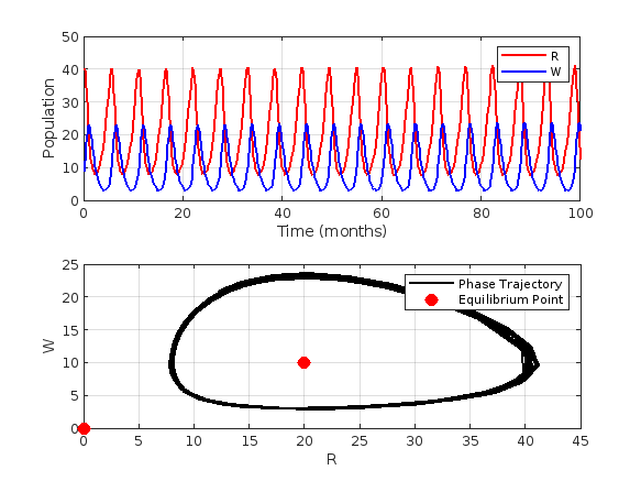
This project discusses predator-prey system, particularly the Lotka-Volterra equations,which model the interaction between two sprecies: prey and predators. Let's solve the Lotka-Volterra equations numerically and visualize the results.% Define parameters
% Define parameters
alpha = 1.0; % Prey birth rate
beta = 0.1; % Predator success rate
gamma = 1.5; % Predator death rate
delta = 0.075; % Predator reproduction rate
% Define the symbolic variables
syms R W
% Define the equations
eq1 = alpha * R - beta * R * W == 0;
eq2 = delta * R * W - gamma * W == 0;
% Solve the equations
equilibriumPoints = solve([eq1, eq2], [R, W]);
% Extract the equilibrium point values
Req = double(equilibriumPoints.R);
Weq = double(equilibriumPoints.W);
% Display the equilibrium points
equilibriumPointsValues = [Req, Weq]
% Solve the differential equations using ode45
lotkaVolterra = @(t,Y)[alpha*Y(1)-beta*Y(1)*Y(2);
delta*Y(1)*Y(2)-gamma*Y(2)];
% Initial conditions
R0 = 40;
W0 = 9;
Y0 = [R0, W0];
tspan = [0, 100];
% Solve the differential equations
[t, Y] = ode45(lotkaVolterra, tspan, Y0);
% Extract the populations
R = Y(:, 1);
W = Y(:, 2);
% Plot the results
figure;
subplot(2,1,1);
plot(t, R, 'r', 'LineWidth', 1.5);
hold on;
plot(t, W, 'b', 'LineWidth', 1.5);
xlabel('Time (months)');
ylabel('Population');
legend('R', 'W');
grid on;
subplot(2,1,2);
plot(R, W, 'k', 'LineWidth', 1.5);
xlabel('R');
ylabel('W');
grid on;
hold on;
plot(Req, Weq, 'ro', 'MarkerSize', 8, 'MarkerFaceColor', 'r');
legend('Phase Trajectory', 'Equilibrium Point');
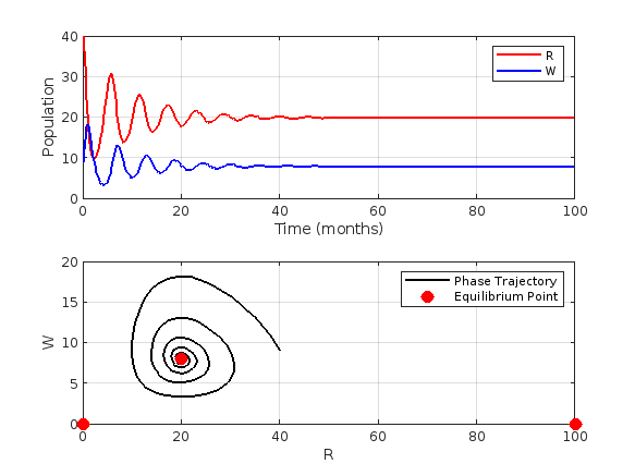
Now, we need to handle a modified version of the Lotka-Volterra equations. These modified equations incorporate logistic growth fot the prey population.
These equations are:


% Define parameters
alpha = 1.0;
K = 100; % Carrying Capacity of the prey population
beta = 0.1;
gamma = 1.5;
delta = 0.075;
% Define the symbolic variables
syms R W
% Define the equations
eq1 = alpha*R*(1 - R/K) - beta*R*W == 0;
eq2 = delta*R*W - gamma*W == 0;
% Solve the equations
equilibriumPoints = solve([eq1, eq2], [R, W]);
% Extract the equilibrium point values
Req = double(equilibriumPoints.R);
Weq = double(equilibriumPoints.W);
% Display the equilibrium points
equilibriumPointsValues = [Req, Weq]
% Solve the differential equations using ode45
modified_lv = @(t,Y)[alpha*Y(1)*(1-Y(1)/K)-beta*Y(1)*Y(2);
delta*Y(1)*Y(2)-gamma*Y(2)];
% Initial conditions
R0 = 40;
W0 = 9;
Y0 = [R0, W0];
tspan = [0, 100];
% Solve the differential equations
[t, Y] = ode45(modified_lv, tspan, Y0);
% Extract the populations
R = Y(:, 1);
W = Y(:, 2);
% Plot the results
figure;
subplot(2,1,1);
plot(t, R, 'r', 'LineWidth', 1.5);
hold on;
plot(t, W, 'b', 'LineWidth', 1.5);
xlabel('Time (months)');
ylabel('Population');
legend('R', 'W');
grid on;
subplot(2,1,2);
plot(R, W, 'k', 'LineWidth', 1.5);
xlabel('R');
ylabel('W');
grid on;
hold on;
plot(Req, Weq, 'ro', 'MarkerSize', 8, 'MarkerFaceColor', 'r');
legend('Phase Trajectory', 'Equilibrium Point');