다음에 대한 결과:
- New cross-platform MCP Bundle; one-click installation in Claude Desktop
- Provide structured output from check_matlab_code and additional information for MATLAB R2022b onwards
- Made project_path optional in evaluate_matlab_code tool for simpler tool calls
- Enhanced detect_matlab_toolboxes output to include product version
- Updated MCP Go SDK dependency to address CVE.
- Added Plain Text Live Code Guidelines MCP resource
- Added MCP Annotations to all tools

- Address Readers’ Needs:
- Enhance Authors’ Experience:
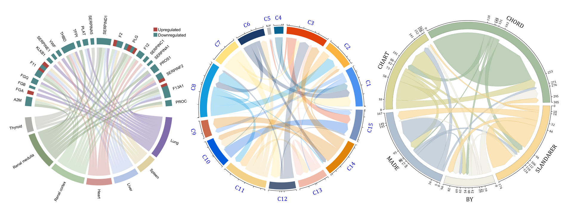
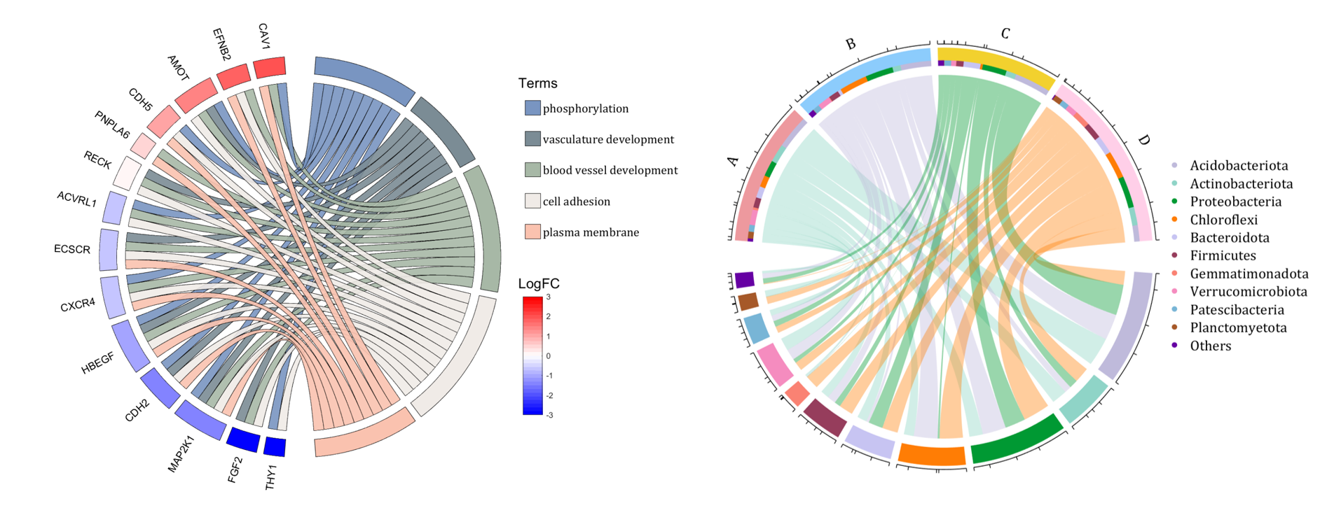
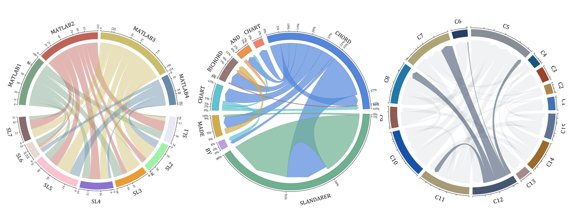
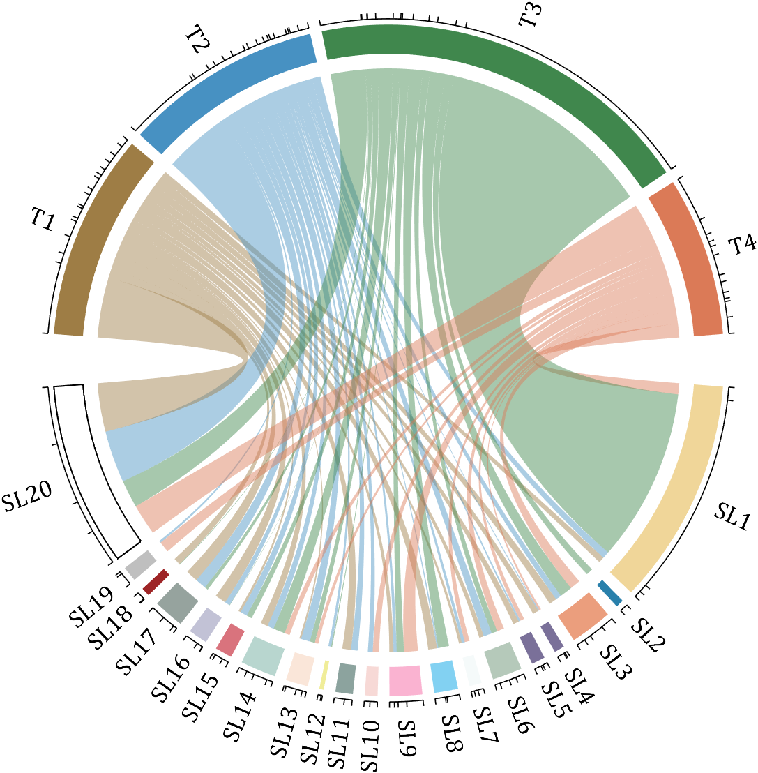
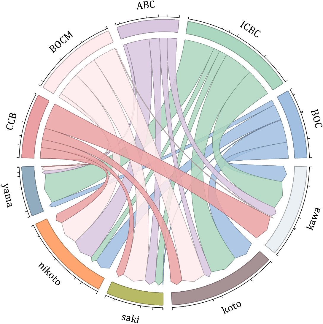
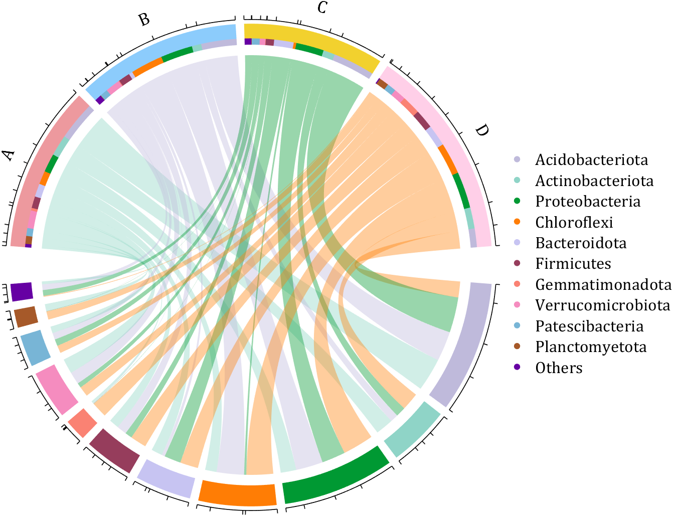
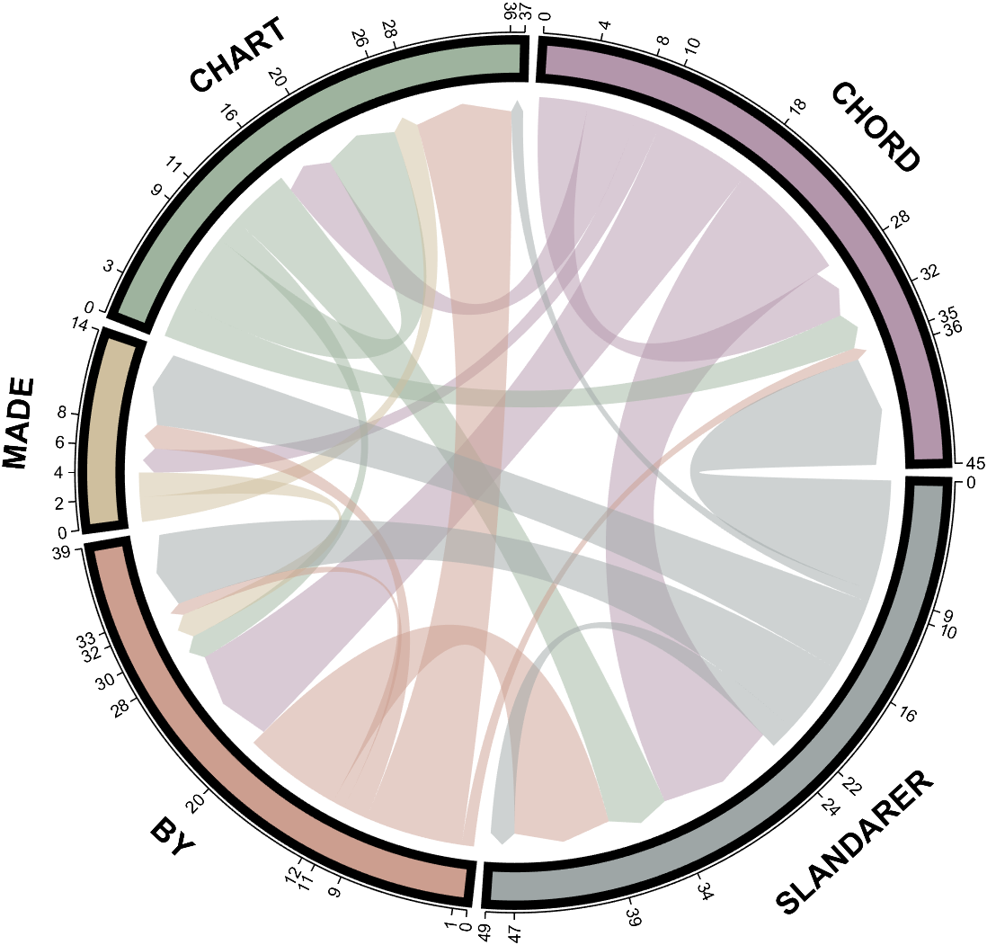
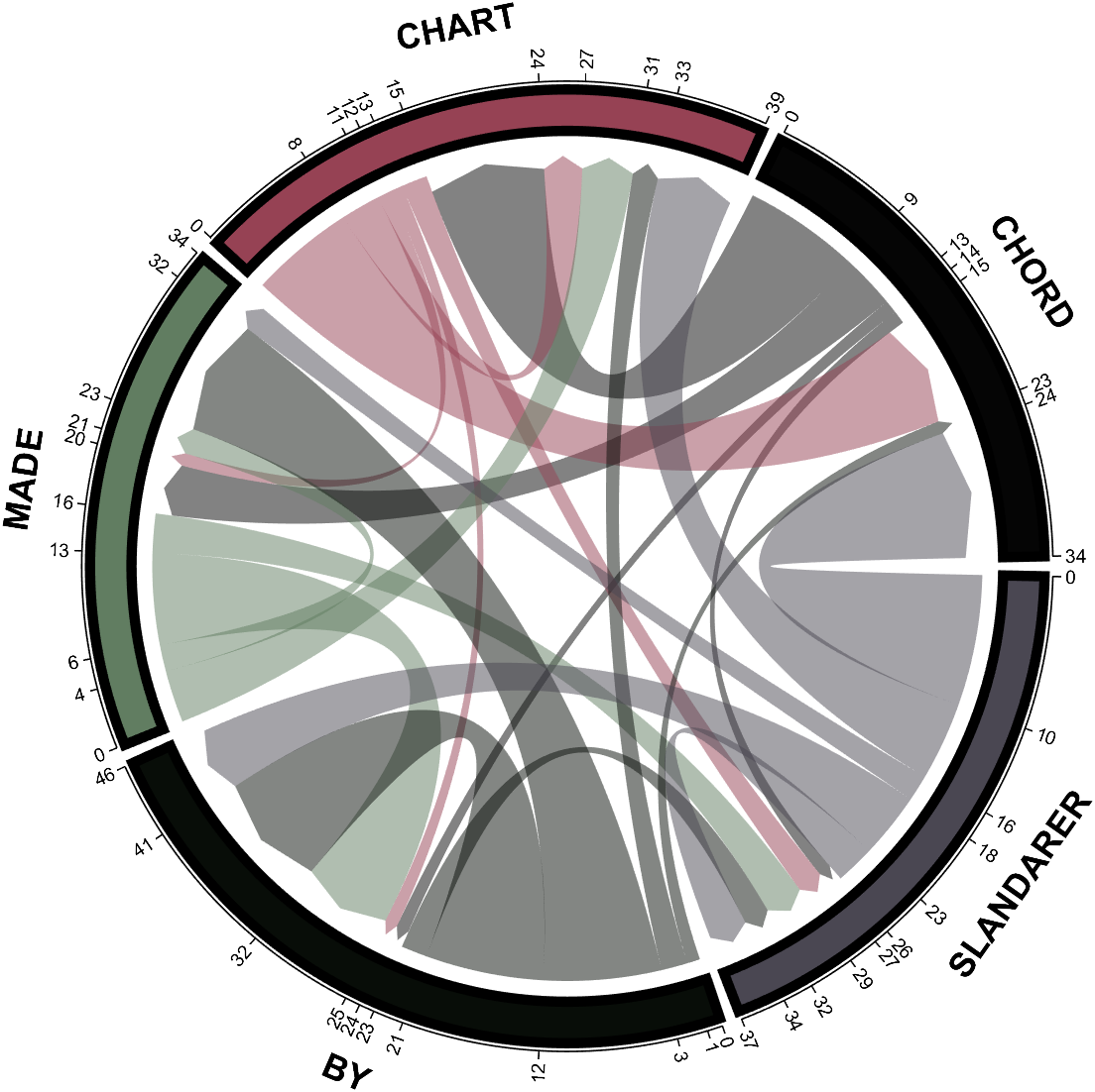
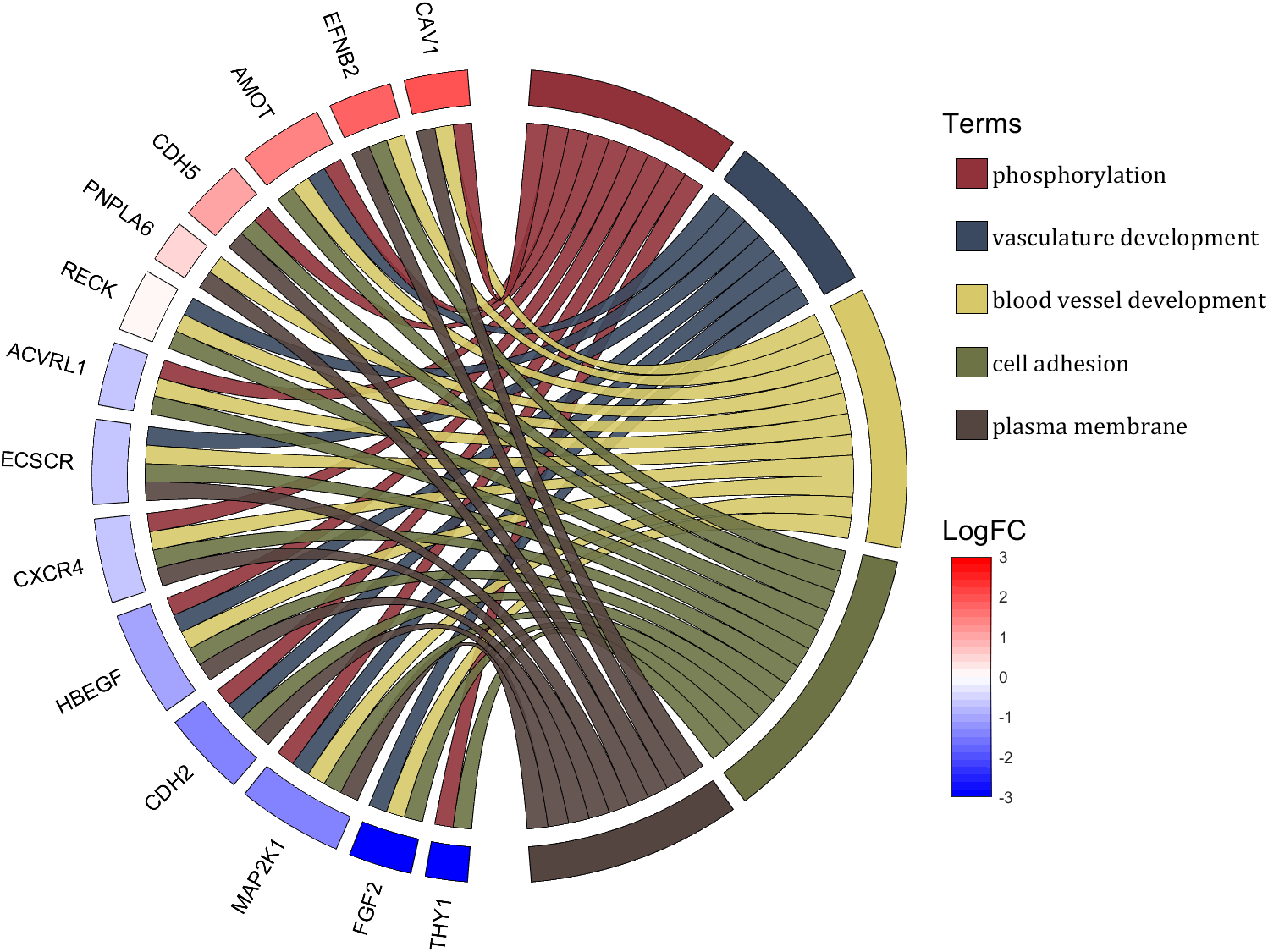
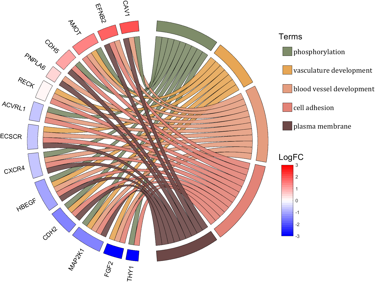
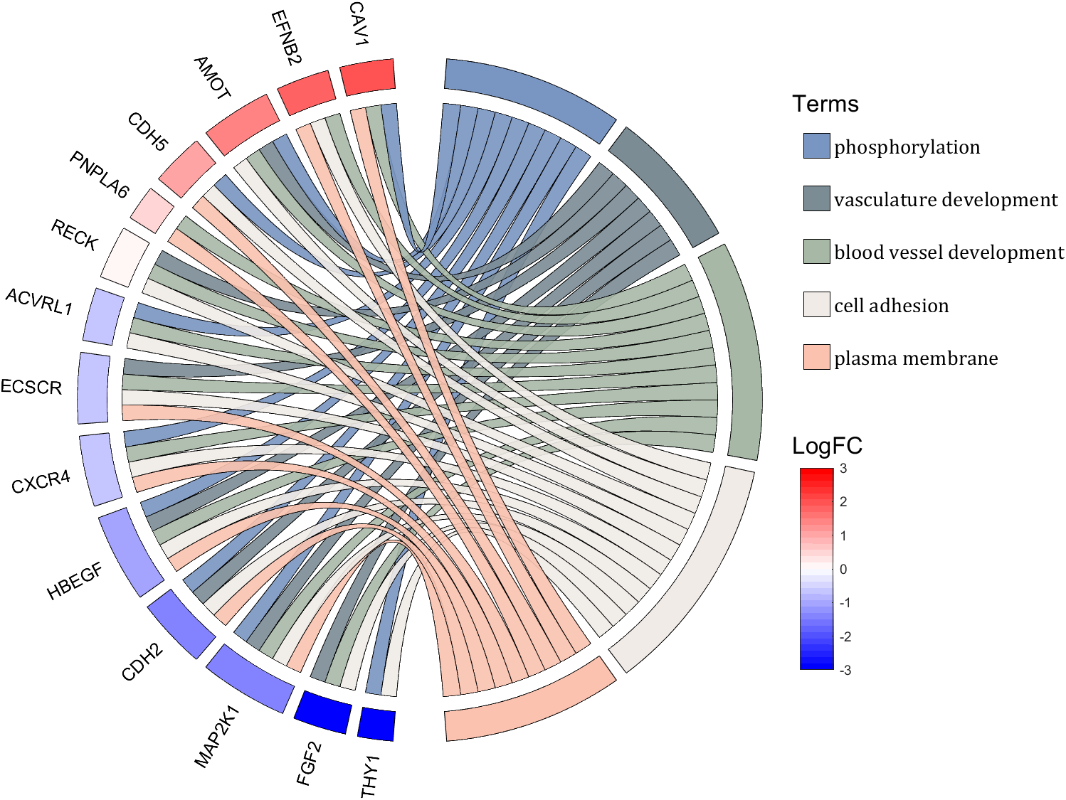
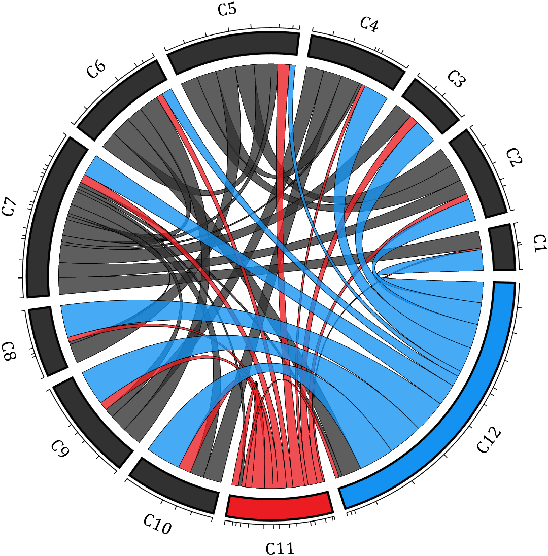
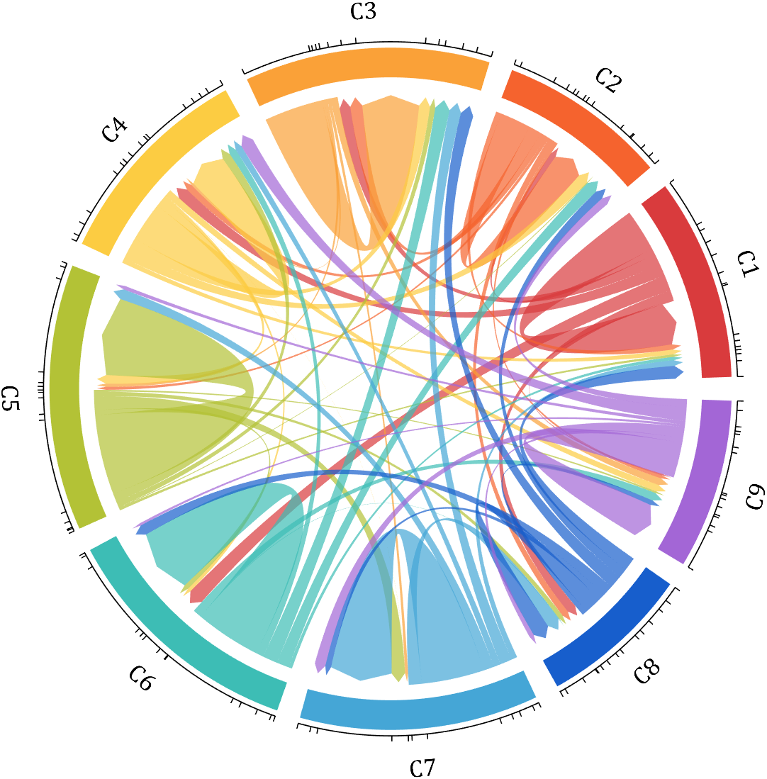
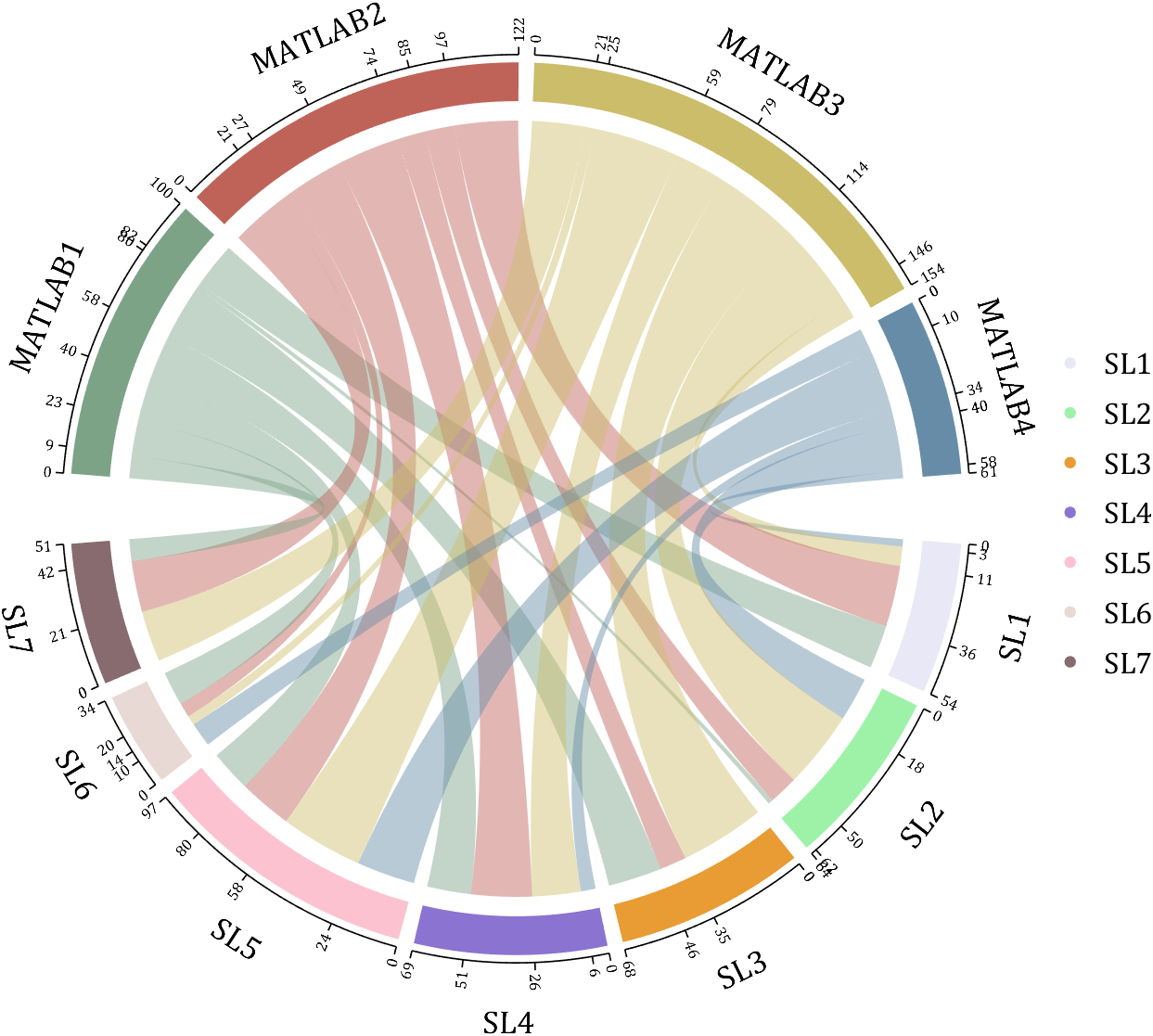
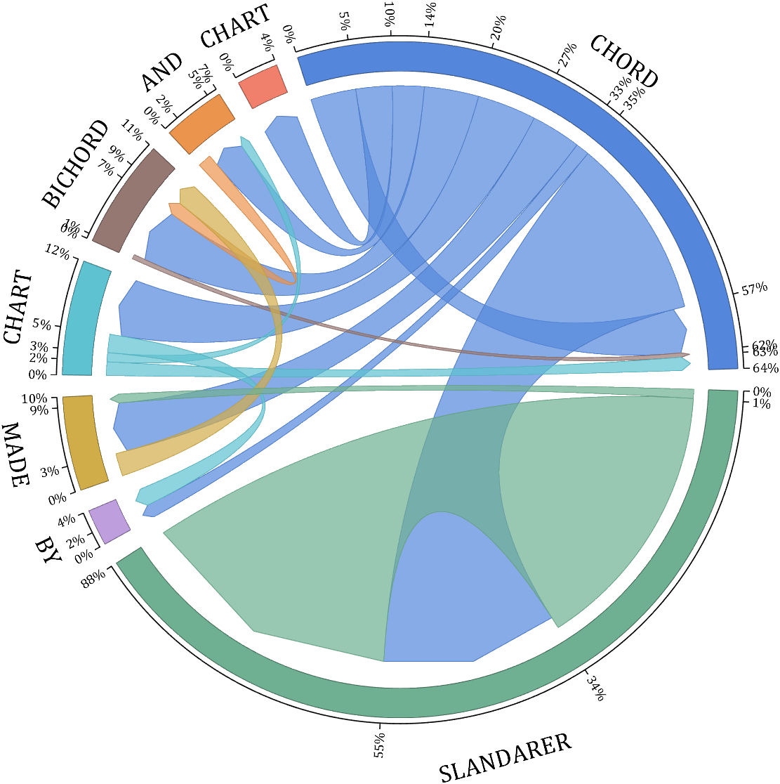
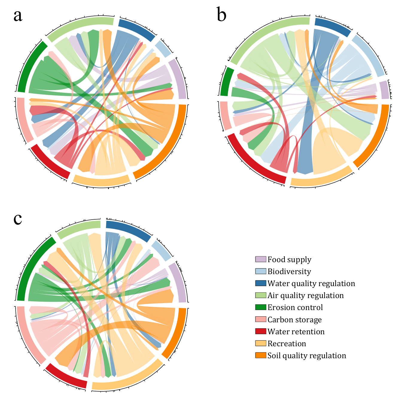
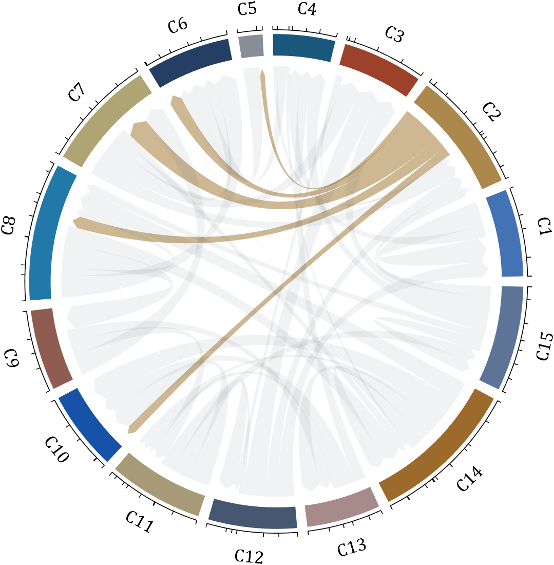
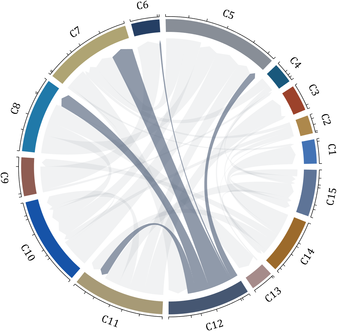
- - Chord chart: [chord chart](https://www.mathworks.com/matlabcentral/fileexchange/116550-chord-chart)
- - Directed graph chord chart: [digraph chord chart]:(https://www.mathworks.com/matlabcentral/fileexchange/121043-digraph-chord-chart)
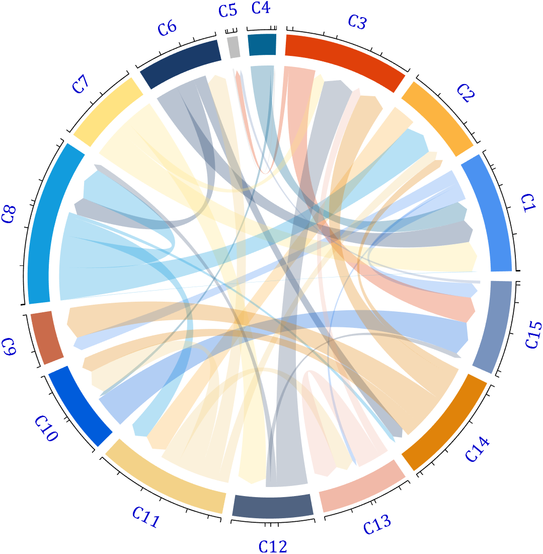
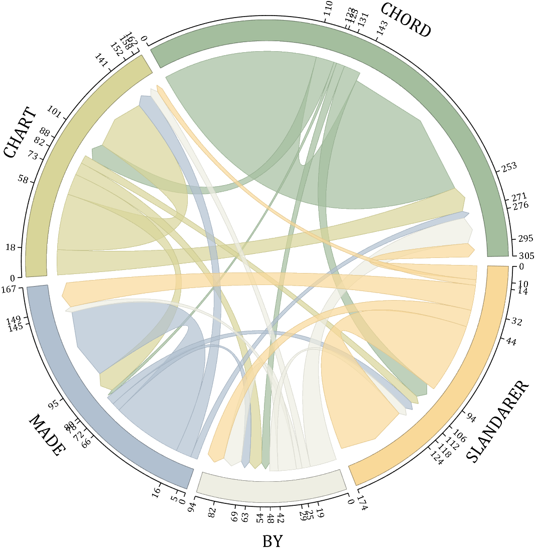
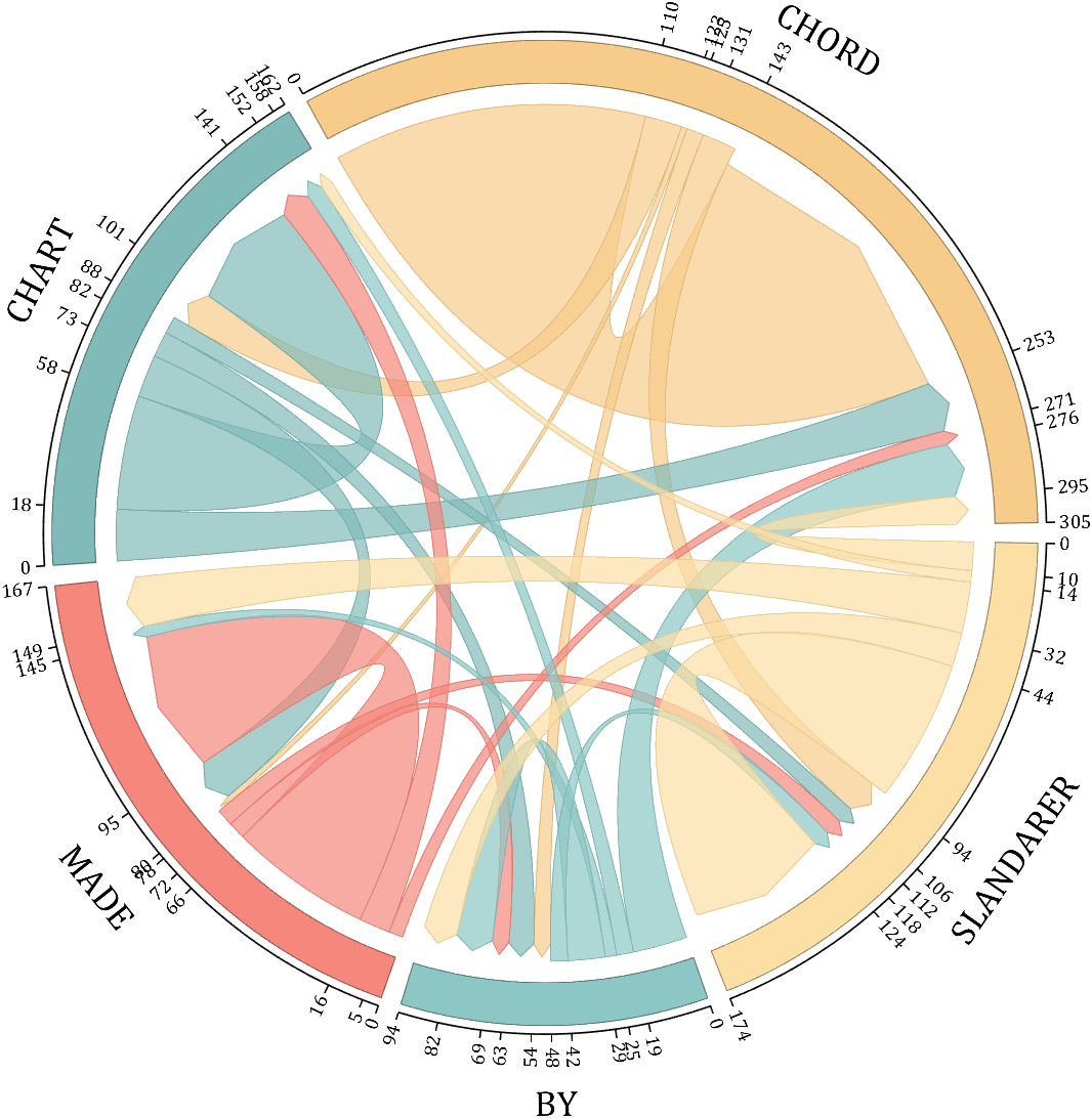
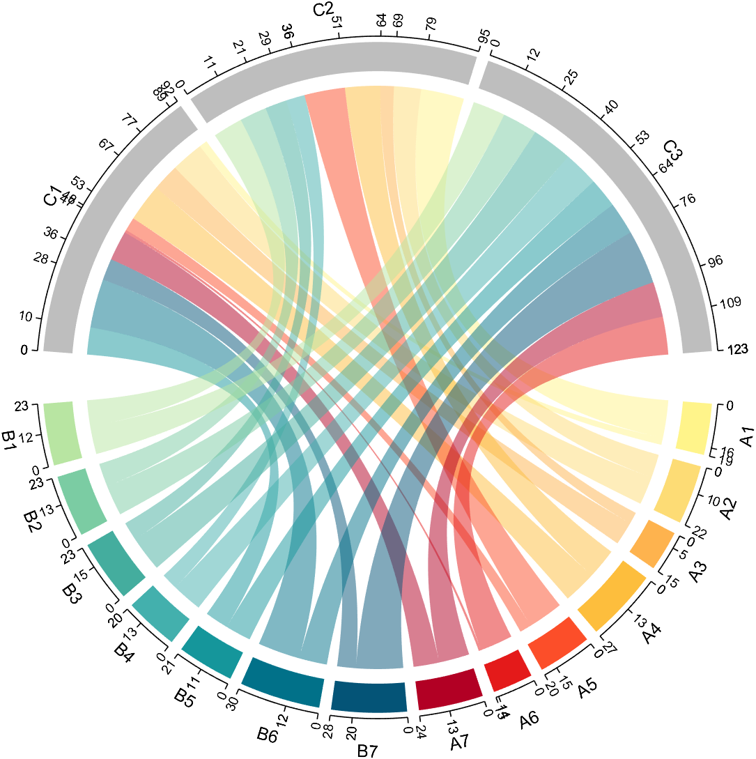
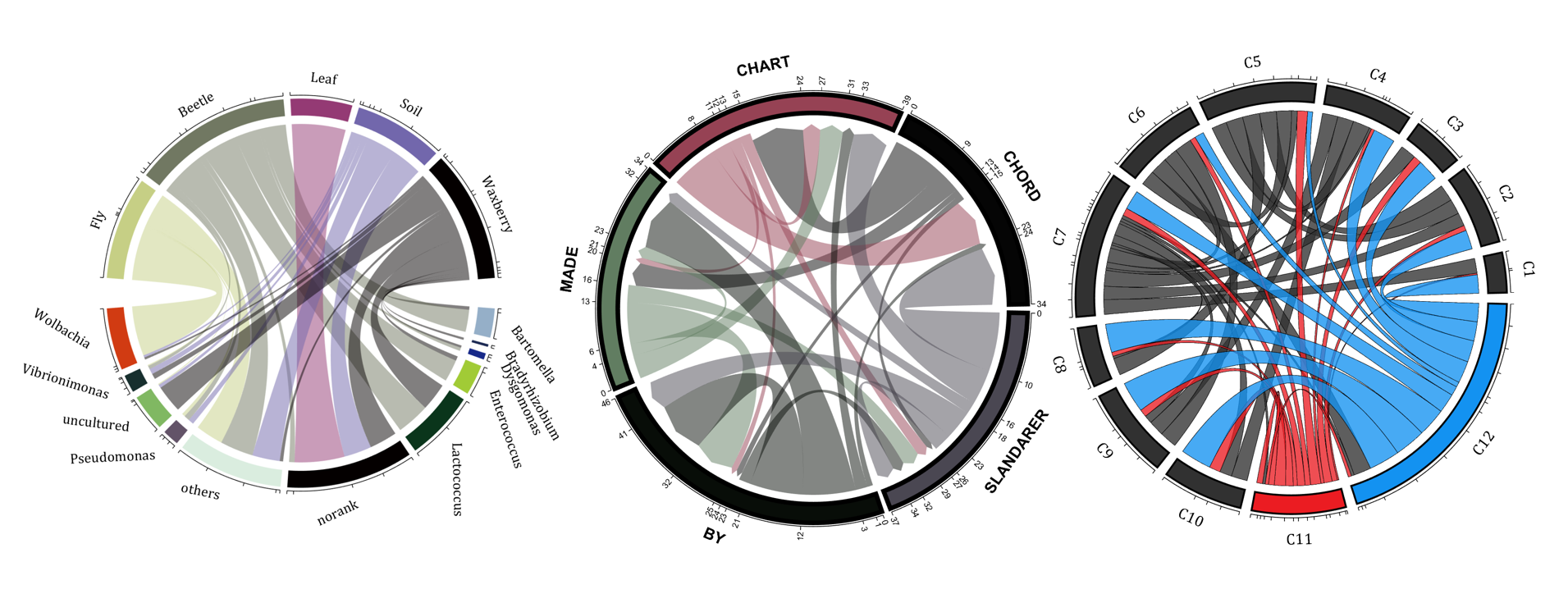
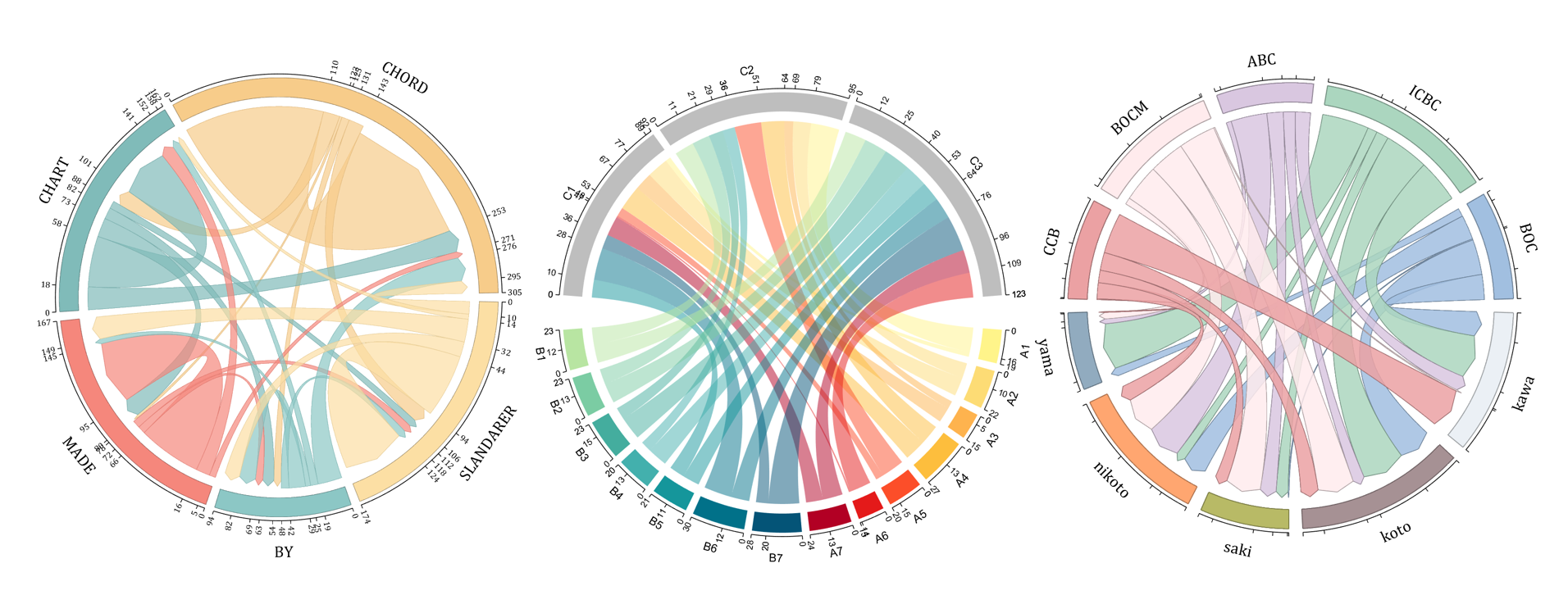
- - Chord chart: [chord chart](https://www.mathworks.com/matlabcentral/fileexchange/116550-chord-chart)
- - Directed graph chord chart: [digraph chord chart]:(https://www.mathworks.com/matlabcentral/fileexchange/121043-digraph-chord-chart)
20 minutes makes a difference
I struggled to learn MATLAB at first. A colleague at my university gave me about 20 minutes of his time to show me some basic features, how to reference the documentation, and how to debug code. That was enough for me to start using MATLAB independently. After a few semesters of developing analyses and visualizations, I started answering questions in the forum when I had time. I became addicted to volunteering and learning from the breadth of analytical problems the forum exposed me to.
Have you ever solved a problem using a MathWorks product?
If your answer is YES, you may be the right person to help someone looking for guidance to solve a similar problem. Some answers in the MATLAB Central community forum maintain 1000s of views per month and some files on the File Exchange have 1000s of downloads. Volunteering a moment of your time to answer a question or to share content to the File Exchange may benefit countless individuals in the near and distant future and you will likely learn a lot by contributing too!
- 3616 questions were asked last month in the forum and in that time, 747 volunteers answered at least one question!
- 62% of those volunteers were first-time contributors!
- 335 volunteer contributors shared content in the File Exchange last month!
- 1: the number of contributions it takes to make a difference.
This week is National Volunteer Week in the USA (April 17-23). Challenge yourself and your colleagues by committing to help a stranger break barriers in their path to learning MATLAB.
How to volunteer and contribute to the MATLAB Central Community
Here are two easy ways to accept the volunteer challenge.
Contribute to the MATLAB Answers Forum
- Go to the MATLAB Answers repository. This page shows all unanswered questions starting with the most recent question. Use the filters on the left to see answered questions or questions belonging to a specific category. Alternatively, search for questions using keywords in the search field or visit the landing page.
- Open a few questions that interest you based on the question titles and tags.
- Decide how you'd like to contribute. Sometimes a question needs refinement or requires a bit of work to address. Decide whether to leave a comment that guides the user in the right direction, answer the question, or skip to the next question. The decision tree below is how some experienced contributors approach these decisions.
Pro tips
- Newer questions have more traffic and are often answered within an hour or minutes.
- Multiple answers often add valuable alternative perspectives and solutions.
- Sometimes answers aren't accepted or the asker disappears. Be not discouraged. Your answer holds much value.
Contribute to the File Exchange
- Choose a function, script, demo, or toolbox you created that may be helpful to the community.
- Go to the MathWorks File Exchange. Search for submissions that are similar to your idea and decide whether your idea adds value.
- Prepare your code for open-source sharing. The best submissions include brief documentation that explains the purpose of the code, inputs, expected outputs and limitations.
- Use the "Publish your code" button from the link above. This will guide you through the submission process.
Make a difference
No matter what level you are at as a MATLAB developer, you have skills that others around you could benefit from learning. Take the challenge and become a giant.
Let us know about your experience with MATLAB Central volunteers or your experience becoming a MATLAB Central volunteer in the comments below!
Categorical navigation is now available in MATLAB Answers.
- Categories empower you to find, watch, and answer questions by topic and product, rather than product alone.
- Individual answers have been categorized using an AI model written by MathWorks developers. Read more about our method here.
FAQ
1. What if I've bookmarked or subscribed to a product?
The links will continue to work but use a different filter mechanism. We encourage you to try the new category filter, to find more questions in your topic of interest.
2. Can I still select a product on the question?
Yes - and product and tags are factored into the text analytics algorithm. Correcting those fields should improve the nightly categorization.
Categories are also shown in the Help Center.
Check out your favorite topic of interest and let us know how we're doing in the comments below!
Starting in MATLAB R2021a, name-value arguments have a new optional syntax!
A property name can be paired with its value by an equal sign and the property name is not enclosed in quotes.
Compare the comma-separated name,value syntax to the new equal-sign syntax, either of which can be used in >=r2021a:
- plot(x, y, "b-", "LineWidth", 2)
- plot(x, y, "b-", LineWidth=2)
It comes with some limitations:
- It's recommended to use only one syntax in a function call but if you're feeling rebellious and want to mix the syntaxes, all of the name=value arguments must appear after the comma-separated name,value arguments.
- Like the comma-separated name,value arguments, the name=value arguments must appear after positional arguments.
- Name=value pairs must be used directly in function calls and cannot be wrapped in cell arrays or additional parentheses.
Some other notes:
- The property names are not case-sensitive so color='r' and Color='r' are both supported.
- Partial name matches are also supported. plot(1:5, LineW=4)
The new syntax is helpful in distinguishing property names from property values in long lists of name-value arguments within the same line.
For example, compare the following 2 lines:
h = uicontrol(hfig, "Style", "checkbox", "String", "Long", "Units", "Normalize", "Tag", "chkBox1")
h = uicontrol(hfig, Style="checkbox", String="Long", Units="Normalize", Tag="chkBox1")
Here's another side-by-side comparison of the two syntaxes. See the attached mlx file for the full code and all content of this Community Highlight.
We've all been there. You've got some kind of output that displays perfectly in the command window and you just want to capture that display as a string so you can use it again somewhere else. Maybe it's a multidimensional array, a table, a structure, or a fit object that perfectly displays the information you need in a neat and tidy format but when you try to recreate the display in a string variable it's like reconstructing the Taj Mahal out of legos.
Enter Matlab r2021a > formattedDisplayText()
Use str=formattedDisplayText(var) the same way you use disp(var) except instead of displaying the output, it's stored as a string as it would appear in the command window.
Additional name-value pairs allow you to
- Specify a numeric format
- Specify loose|compact line spacing
- Display true|false instead of 1|0 for logical values
- Include or suppress markup formatting that may appear in the display such as the bold headers in tables.
Demo: Record the input table and results of a polynomial curve fit
load census
[fitobj, gof] = fit(cdate, pop, 'poly3', 'normalize', 'on')
Results printed to the command window:
fitobj =
     Linear model Poly3:
     fitobj(x) = p1*x^3 + p2*x^2 + p3*x + p4
       where x is normalized by mean 1890 and std 62.05
     Coefficients (with 95% confidence bounds):
       p1 =       0.921  (-0.9743, 2.816)
       p2 =       25.18  (23.57, 26.79)
       p3 =       73.86  (70.33, 77.39)
       p4 =       61.74  (59.69, 63.8)
gof =
  struct with fields:
             sse: 149.77
         rsquare: 0.99879
             dfe: 17
      adjrsquare: 0.99857
            rmse: 2.9682
Capture the input table, the printed fit object, and goodness-of-fit structure as strings:
rawDataStr = formattedDisplayText(table(cdate,pop),'SuppressMarkup',true)
fitStr = formattedDisplayText(fitobj)
gofStr = formattedDisplayText(gof)
Display the strings:
rawDataStr =
    "    cdate     pop
         _____    _____
         1790       3.9
         1800       5.3
         1810       7.2
         1820       9.6
         1830      12.9
         1840      17.1
         1850      23.1
         1860      31.4
         1870      38.6
         1880      50.2
         1890      62.9
         1900        76
         1910        92
         1920     105.7
         1930     122.8
         1940     131.7
         1950     150.7
         1960       179
         1970       205
         1980     226.5
         1990     248.7
     "
fitStr =
    "     Linear model Poly3:
          ary(x) = p1*x^3 + p2*x^2 + p3*x + p4
            where x is normalized by mean 1890 and std 62.05
          Coefficients (with 95% confidence bounds):
            p1 =       0.921  (-0.9743, 2.816)
            p2 =       25.18  (23.57, 26.79)
            p3 =       73.86  (70.33, 77.39)
            p4 =       61.74  (59.69, 63.8)
     "
gofStr =
    "           sse: 149.77
            rsquare: 0.99879
                dfe: 17
         adjrsquare: 0.99857
               rmse: 2.9682
     "
Combine the strings into a single string and write it to a text file in your temp directory:
txt =  strjoin([rawDataStr; fitStr; gofStr],[newline newline]);
file = fullfile(tempdir,'results.txt');
fid = fopen(file,'w+');
cleanup = onCleanup(@()fclose(fid));
fprintf(fid, '%s', txt);
clear cleanup
Open results.txt.
winopen(file) % for Windows platforms
MATLAB Answers will now properly handle the use of the '*@*' character when you want to get someone's attention. This behavior is commonly referred to as 'mentioning' or 'tagging' someone and is a feature found in most communication apps.
Why we are doing this
To help with communication and potentially speed up conversations. Also, it turns out many of you have been typing the @ character in Answers already, even though the MATLAB Answers site didn't behave in the expected way.
How it works
Once you type the @ character a popup will appear listing the community members already in the Q/A thread, as you keep typing the list will expand to include members not in the thread. A mentioned user will receive a notification when the question/answer/comment is posted. Each mention in the Q/A thread will have a new visual style and link to the user profile for that community member.
If you don't want to get 'mentioned' you can turn off the setting in your communication preferences located on your profile page .
We hope you will find this feature helpful and as always please reply with any feedback you may have.
- Use the new exportapp function to capture an image of your app|uifigure
- MATLAB's getframe now supports apps & uifigures
- Review: How to get the handle to an app figure
Use the new exportapp function to capture an image of your app|uifigure
Imagine these scenarios:
- Your app contains several adjustable parameters that update an embedded plot and you'd like to remember the values of each app component so that you can recreate the plot with the same dataset
- You're constructing a manual for your app and would like to include images of your app
- You're app contains a process that automatically updates regularly and you'd like to store periodic snapshots of your app.
As of MATLABs R2020b release , we no longer must rely on 3rd party software to record an image of an app or uifigure.
exportapp(fig,filename) saves an image (JPEG | PNG | TIFF | PDF) of a uifigure ( fig) with the specified file name or full file path ( filename). MATLAB's documentation includes an example of how to add an [Export] button to an app that allows the user to select a path, filename, and extension for their exported image.
Here's another example that merely saves the image as a PDF to the app's main folder.
1. Add a button to the app and assign a ButtonPushed callback function to the button. This one also assigns an icon to the button in the form of an svg file.

2. Define the callback function to name the image after the app's name and include a datetime stamp. The image will be saved to the app's main folder.
% Button pushed function: SnapshotButton
function SnapshotButtonPushed(app, ~)
    % create filename containing the app's figure name (spaces removed)
    % and a datetime stamp in format yymmdd_hhmmss
    filename = sprintf('%s_%s.pdf',regexprep(app.MyApp.Name,' +',''), datestr(now(),'yymmdd_HHMMSS'));
    % Get the app's path
    filepath = fileparts(which([mfilename,'.mlapp']));
    % Store snapshot
    exportapp(app.MyApp, fullfile(filepath,filename))
end
Matlab's getframe now supports apps & uifigures
getframe(h) captures images of axes or a uifigure as a structure containing the image data which defines a movie frame. This function has been around for a while but as of r2020b , it now supports uifigures. By capturing consecutive frames, you can create a movie that can be played back within a Matlab figure (using movie ) or as an AVI file (using VideoWriter ). This is useful when demonstrating the effects of changes to app components.
The general steps to recording a process within an app as a movie are,
1. Add a button or some other event to your app that can invoke the frame recording process.
2. Animation is typically controlled by a loop with n iterations. Preallocate the structure array that will store the outputs to getframe. The example below stores the outputs within the app so that they are available by other functions within the app. That will require you to define the variable as a property in the app.
% nFrames is the number of iterations that will be recorded.
% recordedFrames is defined as a private property within the app
app.recordedFrames(1:nFrames) = struct('cdata',[],'colormap',[]);
3. Call getframe from within the loop that controls the animation. If you're using VideoWriter to create an AVI file, you'll also do that here (not shown, but see an example in the documentation ).
% app.myAppUIFigure: the app's figure handle
% getframe() also accepts axis handles
for i = 1:nFrames
... % code that updates the app for the next frame
      app.recordedFrames(i) = getframe(app.myAppUIFigure);
  end
4. Now the frame data are stored in app.recordedFrames and can be accessed from anywhere within the app. To play them back as a movie,
movie(app.recordedFrames)
% or
movie(app.recordedFrames, n) % to play the movie n-times
movie(app.recordedFrames, n, fps) % to specify the number of frames per second
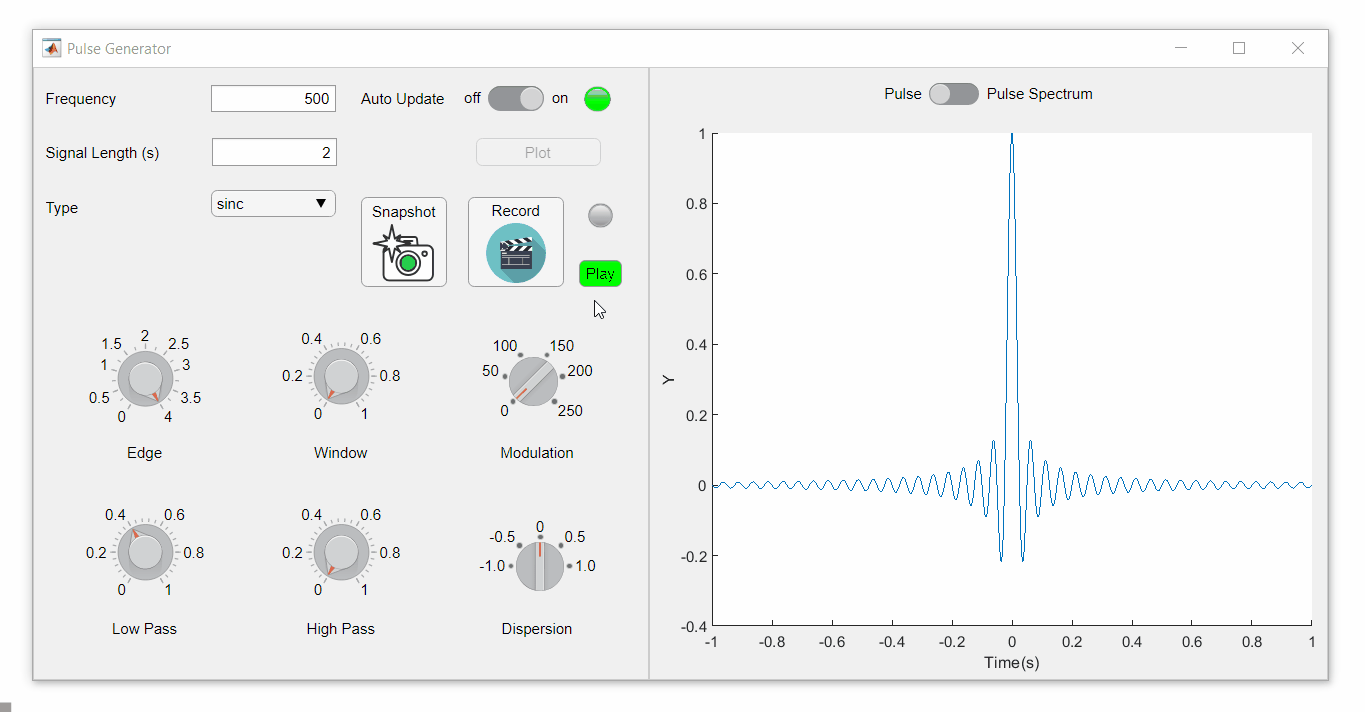
To demonstrate this, I adapted a copy of Matlab's built-in PulseGenerator.mlapp by adding
- a record button
- a record status lamp with frame counter
- a playback button
- a function that animates the effects of the Edge Knob
Recording process (The GIF is a lot faster than realtime and only shows part of the recording) (Open the image in a new window or see the attached Live Script for a clearer image).
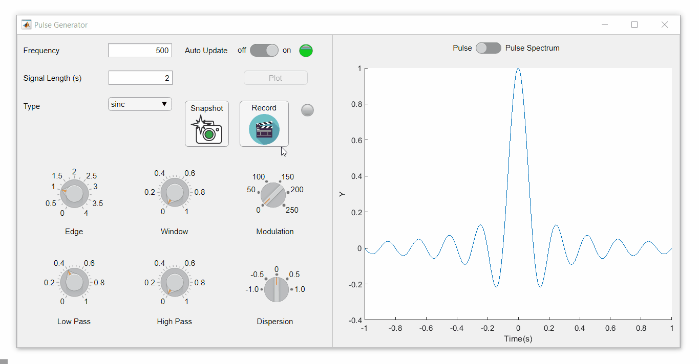
Playback process (Open the image in a new window or see the attached Live Script for a clearer image.)
Review: How to get the handle to an app figure
To use either of these functions outside of app designer, you'll need to access the App's figure handle. By default, the HandleVisibility property of uifigures is set to off preventing the use of gcf to retrieve the figure handle. Here are 4 ways to access the app's figure handle from outside of the app.
1. Store the app's handle when opening the app.
app = myApp;
% Get the figure handle
figureHandle = app.myAppUIFigure;
2. Search for the figure handle using the app's name, tag, or any other unique property value
allfigs = findall(0, 'Type', 'figure'); % handle to all existing figures
figureHandle = findall(allfigs, 'Name', 'MyApp', 'Tag', 'MyUniqueTagName');
3. Change the HandleVisibility property to on or callback so that the figure handle is accessible by gcf anywhere or from within callback functions. This can be changed programmatically or from within the app designer component browser. Note, this is not recommended since any function that uses gcf such as axes(), clf(), etc can now access your app!.
4. If the app's figure handle is needed within a callback function external to the app, you could pass the app's figure handle in as an input variable or you could use gcbf() even if the HandleVisibility is off.
See a complete list of changes to the PulseGenerator app in the attached Live Script file to recreate the app.
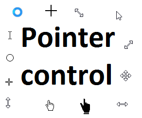
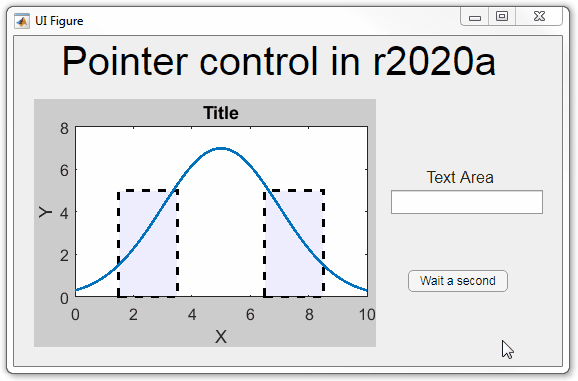
Starting in r2020a , you can change the mouse pointer symbol in apps and uifigures.
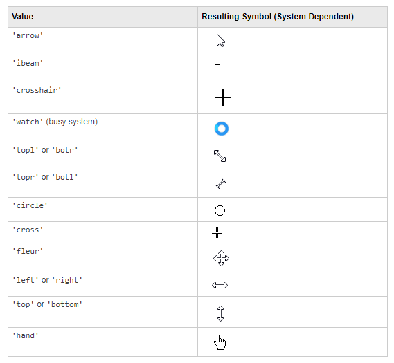
The Pointer property of a figure defines the cursor’s default pointer symbol within the figure. You can also create your own pointer symbols (see part 3, below).
Part 1. How to define a default pointer symbol for a uifigure or app
For figures or uifigures, set the pointer property when you define the figure or change the pointer property using the figure handle.
% Set pointer when creating the figure
uifig = uifigure('Pointer', 'crosshair');
% Change pointer after creating the figure
uifig.Pointer = 'crosshair';
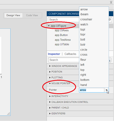
For apps made in AppDesigner, you can either set the pointer from the Design View or you can set the pointer property of the app’s UIFigure from the startup function using the second syntax shown above.
Part 2. How to change the pointer symbol dynamically
The pointer can be changed by setting specific conditions that trigger a change in the pointer symbol.
For example, the pointer can be temporarily changed to a busy-symbol when a button is pressed. This ButtonPushed callback function changes the pointer for 1 second.
function WaitasecondButtonPushed(app, event)
   % Change pointer for 1 second.
   set(app.UIFigure, 'Pointer','watch')
   pause(1)
   % Change back to default.
   set(app.UIFigure, 'Pointer','arrow')
   app.WaitasecondButton.Value = false;
end
The pointer can be changed every time it enters or leaves a uiaxes or any plotted object within the uiaxes. This is controlled by a set of pointer management functions that can be set in the app’s startup function.
iptSetPointerBehavior(obj,pointerBehavior) allows you to define what happens when the pointer enters, leaves, or moves within an object. Currently, only axes and axes objects seem to be supported for UIFigures.
iptPointerManager(hFigure,'enable') enables the figure’s pointer manager and updates it to recognize the newly added pointer behaviors.
The snippet below can be placed in the app’s startup function to change the pointer to crosshairs when the pointer enters the outerposition of a uiaxes and then change it back to the default arrow when it leaves the uiaxes.
% Define pointer behavior when pointer enter axes
pm.enterFcn = @(~,~) set(app.UIFigure, 'Pointer', 'crosshair');
pm.exitFcn  = @(~,~) set(app.UIFigure, 'Pointer', 'arrow');
pm.traverseFcn = [];
iptSetPointerBehavior(app.UIAxes, pm)
% Enable pointer manager for app
iptPointerManager(app.UIFigure,'enable');
Any function can be triggered when entering/exiting an axes object which makes the pointer management tools quite powerful. This snippet below defines a custom function cursorPositionFeedback() that responds to the pointer entering/exiting a patch object plotted within the uiaxes. When the pointer enters the patch, the patch color is changed to red, the pointer is changed to double arrows, and text appears in the app’s text area. When the pointer exits, the patch color changes back to blue, the pointer changes back to crosshairs, and the text area is cleared.
% Plot patch on uiaxes
hold(app.UIAxes, 'on')
region1 = patch(app.UIAxes,[1.5 3.5 3.5 1.5],[0 0 5 5],'b','FaceAlpha',0.07,...
    'LineWidth',2,'LineStyle','--','tag','region1');
% Define pointer behavior for patch
pm.enterFcn = @(~,~) cursorPositionFeedback(app, region1, 'in');
pm.exitFcn  = @(~,~) cursorPositionFeedback(app, region1, 'out');
pm.traverseFcn = [];
iptSetPointerBehavior(region1, pm)
% Enable pointer manager for app
iptPointerManager(app.UIFigure,'enable');
function cursorPositionFeedback(app, hobj, inout)
% When inout is 'in', change hobj facecolor to red and update textbox.
% When inout is 'out' change hobj facecolor to blue, and clear textbox.
% Check tag property of hobj to identify the object.
switch lower(inout)
    case 'in'
        facecolor = 'r';
        txt = 'Inside region 1';
        pointer = 'fleur';
    case 'out'
        facecolor = 'b';
        txt = '';
        pointer = 'crosshair';
end
hobj.FaceColor = facecolor;
app.TextArea.Value = txt;
set(app.UIFigure, 'Pointer', pointer)
end
The app showing the demo below is attached.
Part 3. Create your own custom pointer symbol
- Set the figure’s pointer property to ‘custom’.
- Set the figure’s PointerShapeCData property to the custom pointer matrix. A custom pointer is defined by a 16x16 or 32x32 matrix where NaN values are transparent, 1=black, and 2=white.
- Set the figure’s PointerShapeHotSpot to [m,n] where m and n are the coordinates that define the tip or "hotspot" of the matrix.
This demo uses the attached mat file to create a black hand pointer symbol.
iconData = load('blackHandPointer.mat');
uifig = uifigure();
uifig.Pointer = 'custom';
uifig.PointerShapeCData = iconData.blackHandIcon;
uifig.PointerShapeHotSpot = iconData.hotspot;
Also see Jiro's pointereditor() function on the file exchange which allows you to draw your own pointer.