Calibrate Object Detection Confidence Scores
This example shows how to calibrate the confidence scores of an object using Platt scaling.
Platt scaling is an effective post-processing method for converting raw detector confidence scores into well-calibrated probability estimates. This is especially important when detector scores do not represent true probabilities, since proper calibration improves decision thresholds and supports downstream tasks such as object tracking or combining outputs from multiple models in ensemble methods.
In this example, you apply Platt scaling by using logistic regression to map raw detection scores to calibrated probabilities. Then, you visualize calibrated detection scores for individual images to assess how well the calibrated probabilities align with true detections on a per-image basis. This approach improves the interpretability and reliability of detection outputs.
This example requires the Statistics and Machine Learning Toolbox™.
Load Image Test Data
Load the test data set, which consists of images of vehicles on United States highways, and the ground-truth annotations of bounding boxes for vehicle objects.
data = load("vehicleTrainingData.mat");
testData = data.vehicleTrainingData;
Specify dataDir as the location of the data set.
dataDir = fullfile(toolboxdir("vision"),"visiondata");
testData.imageFilename = fullfile(dataDir,testData.imageFilename);
Create an imageDatastore object that stores the image data, and a boxLabelDatastore object that contains the ground truth annotation data for bounding boxes.
imds = imageDatastore(testData.imageFilename);
blds = boxLabelDatastore(testData(:,2:end));
numImages = numel(imds.Files);
Load Object Detector
Load a pretrained YOLOv2 vehicle detector.
vehicleDetector = load("yolov2VehicleDetector.mat");
detector = vehicleDetector.detector;
Detect Objects in Test Images
Predict the mask, labels, and confidence scores for each object instance using the detect object function. To ensure a high recall for detected objects, specify Threshold as 0.1 to set a low score confidence threshold. Optionally, you can filter the detections to reduce false positives that may arise from setting such a low threshold on the score.
results = detect(detector,imds,Threshold=0.1);
Summarize Detector Performance Metrics
Evaluate the detector’s performance on the test set using Average Precision (AP) at multiple IoU thresholds by using the evaluateObjectDetection function. Display the metrics summary across the data set.
metrics = evaluateObjectDetection(results,blds,[0.5 0.7 0.9]);
disp(summarize(metrics))
    NumObjects    mAPOverlapAvg    mAP0.5     mAP0.7      mAP0.9
    __________    _____________    _______    _______    ________

       336           0.60542       0.99096    0.79233    0.032975
These metrics provide a baseline for accuracy before calibration. Note that calibrating confidence scores with Platt scaling does not affect AP values, but improves how well the scores represent the true likelihood of correct detections. In the following sections, you will calibrate the detector’s confidence scores to enhance their reliability.
Analyze Detection Confidence Score Distributions
To effectively evaluate and calibrate the reliability of the model’s confidence estimates, use the detector confidence scores for correct (true positive) and incorrect (false positive) predictions. A positive prediction is defined as one where the overlap with the ground truth exceeds the Intersection over Union (IoU) threshold, indicating a true positive (TP). A negative prediction is defined as one where the overlap with the ground truth is less than or equal to the IoU threshold, indicating a false positive (FP). Set these criteria based on the requirements of your specific application.
Set the overlap threshold between the predicted and ground-truth bounding boxes, IOU_THRESH, to 0.5 for a reasonable level of localization accuracy. This threshold determines whether a predicted bounding box is a true positive.
IOU_THRESH = 0.5;
Set the score threshold, SCORE_THRESH, to 0.1. The score threshold determines the minimum confidence score that a predicted bounding box must have to be included in the evaluation.
SCORE_THRESH = 0.1;
Initialize containers to separately store the positive and negative confidence scores for each result in the dataset.
positiveScores = cell(height(results),1);
negativeScores = cell(height(results),1);
Iterate through each detection result, filtering out low-confidence predictions and calculating the overlap (IoU) between each remaining predicted box and the ground truth boxes. Then, separate the confidence scores into positives and negatives based on whether the IoU exceeds the specified threshold, and finally concatenate all positive and negative confidence scores across the data set.
reset(blds);
for i = 1:height(results)
    gt = read(blds);
    gtBoxes = gt{1};
    predBoxes = results.Boxes{i};
    predScores = results.Scores{i};
    sel = predScores > SCORE_THRESH;
    predBoxes = predBoxes(sel,:);
    predScores = predScores(sel);

    iouMat = bboxOverlapRatio(predBoxes,gtBoxes);
    iouMat = max(iouMat,[],2);

    selPositive = iouMat > IOU_THRESH;

    positiveScores{i} = predScores(selPositive);
    negativeScores{i} = predScores(~selPositive);
end

positiveScores = cat(1,positiveScores{:});
negativeScores = cat(1,negativeScores{:});
Plot a histogram of the positive and negative confidence score distribution.
histBins = [0:0.01:1];
figure; histogram(positiveScores,histBins)
hold on; histogram(negativeScores,histBins)
title("Raw Score Histograms")
xlabel("Score")
ylabel("Frequency")
grid on

Display the number of positive and negative detections.
numPositives = numel(positiveScores)
numPositives =
393
numNegatives = numel(negativeScores)
numNegatives =
1353
Calibrate Detection Confidence Scores Using Platt Scaling
In this section, you calibrate the object detector’s confidence scores using Platt scaling. First, you rescale the positive and negative labels to reduce overfitting, then fit a logistic regression model to map raw scores to calibrated probabilities. Finally, you visualize the calibration mapping and compare the score distributions before and after calibration to assess the effectiveness of the process.
Rescale Detection Scores
To reduce the risk of overfitting during calibration, adjust the positive and negative labels from the standard 0 and 1 values to smoothed values, as suggested by Niculescu-Mizil and Caruana [1]. Set the positive and negative labels such that the label vector y contains these smoothed values for each positive and negative example, respectively.
ypos = (numPositives + 1)./(numPositives + 2);
yneg = 1./(numNegatives + 2);
y = [ypos*ones(numPositives,1);yneg*ones(numNegatives,1)];
Fit Platt Scaling Model
Concatenate the positive and negative confidence scores into a single vector and create a corresponding label vector, where positive scores are labeled as 1 (true positives) and negative scores as 0 (false positives). Then, fit a univariate logistic regression model using the fitglm (Statistics and Machine Learning Toolbox) function. Use the confidence scores as the predictor and the labels as the response variable [1][2]. To learn more, see the i-vector Score Calibration (Audio Toolbox) example.
scoresRaw = [positiveScores;negativeScores];
mdl = fitglm(scoresRaw,y,Distribution="binomial");
Visualize Platt Scaling Mapping
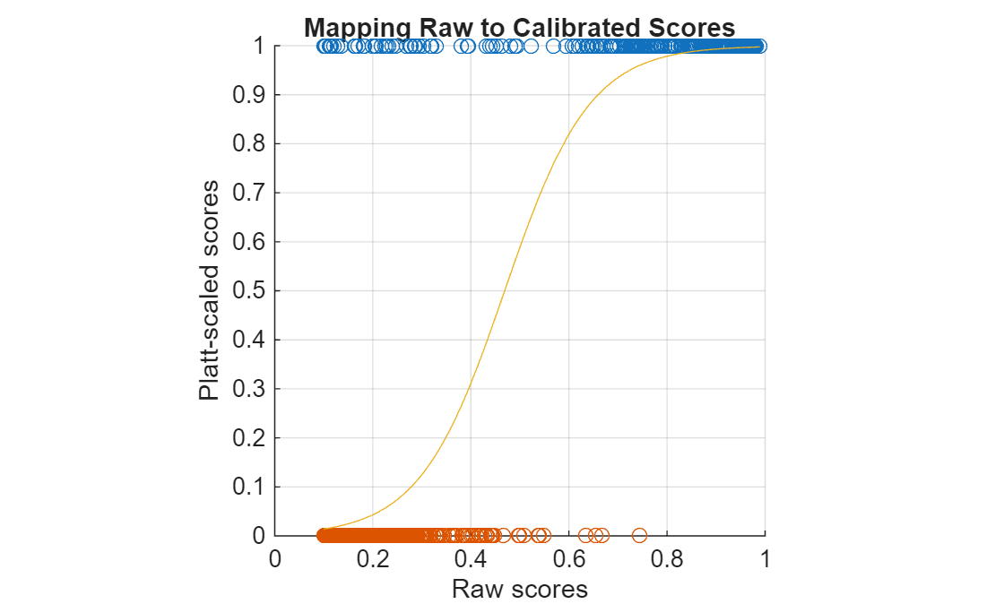
Apply the logistic regression model to the raw detector confidence scores to produce calibrated scores that better reflect the true probability of a correct detection (using the sigmoid mapping learned during Platt scaling).
Then, visualize the relationship between the raw and calibrated scores.
scoresCalib = mdl.predict(scoresRaw);
figure
hold on
Plot the original positive and negative detections as points at 1 and 0, respectively
plot(positiveScores,ones(numPositives,1),"o")
plot(negativeScores,zeros(numNegatives,1),"o")
Overlay the learned sigmoid curve that maps raw scores to their calibrated values.
plot(sort(scoresRaw),sort(scoresCalib),"-")
grid on

xlabel("Raw scores")
ylabel("Platt-scaled scores")
xlim([0 1])
ylim([0 1])
axis("square")
title("Mapping Raw to Calibrated Scores")
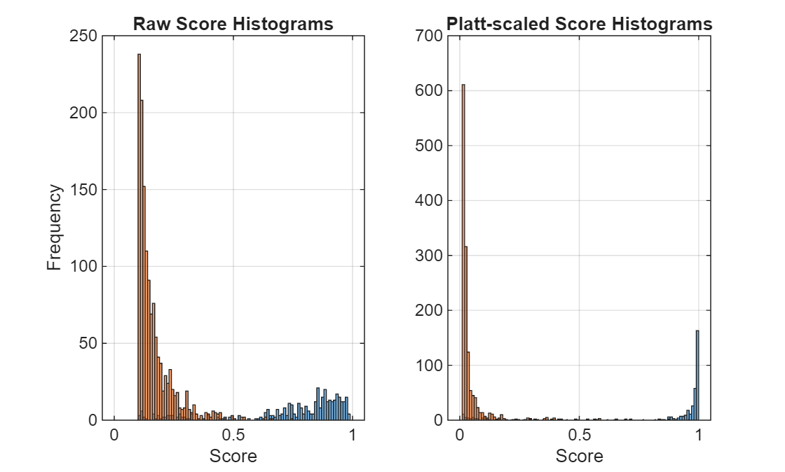
Compare Score Distributions Before and After Calibration
Plot the distributions of detector scores for positives and negatives before and after calibration.
After Platt scaling, the calibrated scores more accurately represent the probability that a detection is a true positive, resulting in improved score calibration compared to the raw outputs.
histBins = [0:0.01:1];
figure
subplot(1,2,1)
histogram(positiveScores,histBins)
hold on; histogram(negativeScores, histBins)
title("Raw Score Histograms")
xlabel("Score")
ylabel("Frequency")
grid on

subplot(1,2,2)
histogram(scoresCalib(1:numPositives),histBins)
hold on; histogram(scoresCalib(numPositives+1:end), histBins)
title("Platt-scaled Score Histograms")
xlabel("Score")
grid on
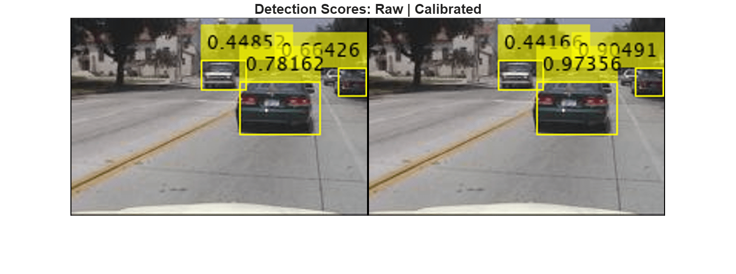
Visualize Calibrated Detection Scores Per Image
Run the detector on a sample image and display the detection confidence scores both before and after Platt scaling. Adjust the slider to choose a different image for which to display the detections and confidence scores.
The visualization shows the original scores and their calibrated counterparts side by side, illustrating how Platt scaling adjusts the detector’s confidence estimates.
imgIdx =130; img = readimage(imds,imgIdx); [boxes, scores, labels] = detect(detector, img, Threshold=0.4); % Calibrate the raw scores using the Platt scaling logistic regression calibratedScores = mdl.predict(scores); imRaw = insertObjectAnnotation(img, "rectangle", boxes, string(scores)); imCalib = insertObjectAnnotation(img, "rectangle", boxes, string(calibratedScores)); figure; montage({imRaw, imCalib}, BorderSize=[1 2]) title( "Detection Scores: Raw | Calibrated") truesize
References
[1] Niculescu-Mizil, Alexandru, and Rich Caruana. “Predicting Good Probabilities with Supervised Learning.” Proceedings of the 22nd International Conference on Machine Learning - ICML ’05, ACM Press, 2005, 625–32. https://doi.org/10.1145/1102351.1102430.
[2] Guo, Chuan, Geoff Pleiss, Yu Sun, and Kilian Q. Weinberger. “On Calibration of Modern Neural Networks.” arXiv.Org, June 14, 2017. https://arxiv.org/abs/1706.04599v2.
See Also
evaluateObjectDetection | yolov2ObjectDetector