Survivor Functions for Two Groups
This example shows how to find the empirical survivor functions and the parametric survivor functions using the Burr type XII distribution fit to data for two groups.
Step 1. Load and prepare sample data.
Load the sample data.
load('lightbulb.mat')The first column of the data has the lifetime (in hours) of two types of light bulbs. The second column has information about the type of light bulb. 0 indicates fluorescent bulbs whereas 1 indicates the incandescent bulb. The third column has censoring information. 1 indicates censored data, and 0 indicates the exact failure time. This is simulated data.
Create a variable for each light bulb type and also include the censorship information.
fluo = [lightbulb(lightbulb(:,2)==0,1),...
			lightbulb(lightbulb(:,2)==0,3)];
insc = [lightbulb(lightbulb(:,2)==1,1),...
			lightbulb(lightbulb(:,2)==1,3)];
Step 2. Plot estimated survivor functions.
Plot the estimated survivor functions for the two different types of light bulbs.
figure()
[f,x,flow,fup] = ecdf(fluo(:,1),'censoring',fluo(:,2),...
				'function','survivor');
ax1 = stairs(x,f);
hold on
stairs(x,flow,':')
stairs(x,fup,':')
[f,x,flow,fup] = ecdf(insc(:,1),'censoring',insc(:,2),...
				'function','survivor');
ax2 = stairs(x,f,'color','r');
stairs(x,flow,':r')
stairs(x,fup,':r')
legend([ax1,ax2],{'Fluorescent','Incandescent'})
xlabel('Lifetime (hours)')
ylabel('Survival probability')
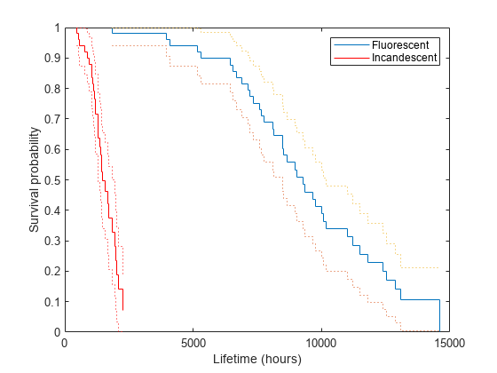
You can see that the survival probability of incandescent light bulbs is much smaller than that of fluorescent light bulbs.
Step 3. Fit Burr Type XII distribution.
Fit Burr distribution to the lifetime data of fluorescent and incandescent type bulbs.
pd = fitdist(fluo(:,1),'burr','Censoring',fluo(:,2))
pd =
  BurrDistribution

  Burr distribution
    alpha = 29143.4   [0.903922, 9.39617e+08]
        c = 3.44582   [2.13013, 5.57417]
        k = 33.7039   [8.10737e-14, 1.40114e+16]
pd2 = fitdist(insc(:,1),'burr','Censoring',insc(:,2))
pd2 =
  BurrDistribution

  Burr distribution
    alpha = 2650.76   [430.773, 16311.4]
        c = 3.41898   [2.16794, 5.39197]
        k =  4.5891   [0.0307809, 684.185]
Superimpose Burr type XII survivor functions.
ax3 = plot(0:500:15000,1-cdf('burr',0:500:15000,29143.5,...
			3.44582,33.704),'m');
ax4 = plot(0:500:5000,1-cdf('burr',0:500:5000,2650.76,...
			3.41898,4.5891),'g');
legend([ax1;ax2;ax3;ax4],'Festimate','Iestimate','FBurr','IBurr')
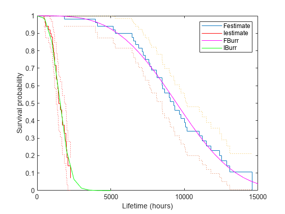
Burr distribution provides a good fit for the lifetime of light bulbs in this example.
Step 4. Fit a Cox proportional hazards model.
Fit a Cox proportional hazards regression where the type of the bulb is the explanatory variable.
[b,logl,H,stats] = coxphfit(lightbulb(:,2),lightbulb(:,1),...
'Censoring',lightbulb(:,3));
stats
stats = struct with fields:
                    covb: 1.0757
                    beta: 4.7262
                      se: 1.0372
                       z: 4.5568
                       p: 5.1936e-06
                   csres: [100×1 double]
                  devres: [100×1 double]
                 martres: [100×1 double]
                  schres: [100×1 double]
                 sschres: [100×1 double]
                  scores: [100×1 double]
                 sscores: [100×1 double]
    LikelihoodRatioTestP: 0
The -value, p, indicates that the type of light bulb is statistically significant. The estimate of the hazard ratio is () = 112.8646. This means that the hazard for the incandescent bulbs is 112.86 times the hazard for the fluorescent bulbs.