plotResiduals
Class: GeneralizedLinearMixedModel
Plot residuals of generalized linear mixed-effects model
Syntax
Description
h = plotResiduals(___)h, to the lines or patches in the plot
of residuals.
Input Arguments
Output Arguments
Examples
Load the sample data.
load mfrThis simulated data is from a manufacturing company that operates 50 factories across the world, with each factory running a batch process to create a finished product. The company wants to decrease the number of defects in each batch, so it developed a new manufacturing process. To test the effectiveness of the new process, the company selected 20 of its factories at random to participate in an experiment: Ten factories implemented the new process, while the other ten continued to run the old process. In each of the 20 factories, the company ran five batches (for a total of 100 batches) and recorded the following data:
Flag to indicate whether the batch used the new process (
newprocess)Processing time for each batch, in hours (
time)Temperature of the batch, in degrees Celsius (
temp)Categorical variable indicating the supplier (
A,B, orC) of the chemical used in the batch (supplier)Number of defects in the batch (
defects)
The data also includes time_dev and temp_dev, which represent the absolute deviation of time and temperature, respectively, from the process standard of 3 hours at 20 degrees Celsius.
Fit a generalized linear mixed-effects model using newprocess, time_dev, temp_dev, and supplier as fixed-effects predictors. Include a random-effects term for intercept grouped by factory, to account for quality differences that might exist due to factory-specific variations. The response variable defects has a Poisson distribution, and the appropriate link function for this model is log. Use the Laplace fit method to estimate the coefficients. Specify the dummy variable encoding as "effects", so the dummy variable coefficients sum to 0.
The number of defects can be modeled using a Poisson distribution:
This corresponds to the generalized linear mixed-effects model
where
is the number of defects observed in the batch produced by factory during batch .
is the mean number of defects corresponding to factory (where ) during batch (where ).
, , and are the measurements for each variable that correspond to factory during batch . For example, indicates whether the batch produced by factory during batch used the new process.
and are dummy variables that use effects (sum-to-zero) coding to indicate whether company
CorB, respectively, supplied the process chemicals for the batch produced by factory during batch .is a random-effects intercept for each factory that accounts for factory-specific variation in quality.
glme = fitglme(mfr,"defects ~ 1 + newprocess + time_dev + temp_dev + supplier + (1|factory)",Distribution="Poisson",Link="log",FitMethod="Laplace",DummyVarCoding="effects");
Create diagnostic plots using Pearson residuals to test the model assumptions.
Plot a histogram to visually confirm that the mean of the Pearson residuals is equal to 0. If the model is correct, we expect the Pearson residuals to be centered at 0.
plotResiduals(glme,"histogram",ResidualType="Pearson")
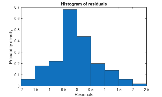
The histogram shows that the Pearson residuals are centered at 0.
Plot the Pearson residuals versus the fitted values, to check for signs of nonconstant variance among the residuals (heteroscedasticity). We expect the conditional Pearson residuals to have a constant variance. Therefore, a plot of conditional Pearson residuals versus conditional fitted values should not reveal any systematic dependence on the conditional fitted values.
plotResiduals(glme,"fitted",ResidualType="Pearson")
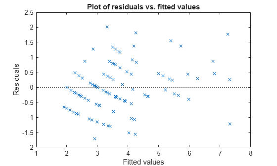
The plot does not show a systematic dependence on the fitted values, so there are no signs of nonconstant variance among the residuals.
Plot the Pearson residuals versus lagged residuals, to check for correlation among the residuals. The conditional independence assumption in GLME implies that the conditional Pearson residuals are approximately uncorrelated.
plotResiduals(glme,"lagged",ResidualType="Pearson")
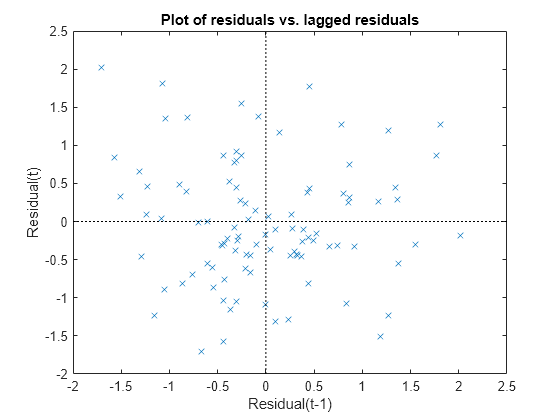
There is no pattern to the plot, so there are no signs of correlation among the residuals.
Version History
See Also
GeneralizedLinearMixedModel | fitglme | fitted | plot | residuals