Compress Machine Learning Model for Memory-Limited Hardware
This example shows how to reduce the size of a machine learning model for deployment to memory-limited hardware. To demonstrate the model compression workflow, the example builds models for the acoustic scene classification (ASC) task, which classifies environments from the sounds they produce. ASC is a generic multiclass classification problem that is foundational for context awareness in devices, robots, and other applications [1].
Assume that you want to build a model for hearing aids where the available memory size is 30 KB. First, simplify the multiclass ASC task to a binary classification problem, and them perform these steps:
Reduce the number of features by selecting important features.
Optimize hyperparameters with coupled constraints, which limit the size of a machine learning model.
Quantize model parameters.
For more details on optimizing hyperparameters to reduce the memory size, see More About.
Load Data
Load the acousticscenes data set, and display the variables in the data set.
load("acousticscenes.mat")
whos
Name Size Bytes Class Attributes xEval 300x286 686400 double xTest 300x286 686400 double xTrain 1500x286 3432000 double yEval 300x1 2102 categorical yTest 300x1 2102 categorical yTrain 1500x1 3302 categorical
xTrain, xEval, and xTest contain features extracted from the TUT acoustic scene data set using wavelet scattering. yTrain, yEval, and yTest contain acoustic scene labels of 15 different types for xTrain, xEval, and xTest, respectively. In this example, you use xTrain and yTrain to train models and xTest and yTest to test the accuracy of the trained models. During the optimization step, you use xEval and yEval as a holdout validation set.
The TUT acoustic scene data set provides development data (TUT-acoustic-scenes-2017-development [3]) and test data (TUT-acoustic-scenes-2017-evaluation [4]). The development data provides a 4-fold cross-validation setup. xTrain and xEval are from the subsets of the training and evaluation sets (respectively) defined by the first fold of the cross-validation setup, and xTest is from the subset of the test data set. The example Acoustic Scene Recognition Using Late Fusion (Audio Toolbox) describes how you can obtain these variables from a subset of the TUT acoustic scene data set.
Normalize the data sets.
[xTrain,mu,sigma] = normalize(xTrain);
xEval = normalize(xEval,center=mu,scale=sigma);
xTest = normalize(xTest,center=mu,scale=sigma);
Select Classification Model Types
Select types of classification models for this example by using the Classification Learner app.
On the Apps tab, open the apps gallery. Then, in the Machine Learning and Deep Learning group, click Classification Learner.
On the Classification Learner tab, in the File section, click New Session and select From Workspace. In the dialog box, specify
yTrainas the response variable, and specify the variables inxTrainas predictors.In the Models section of the app, click All. This option trains all the model presets available for your data set.
In the Train section, click Train All and select Train All.
You can compare trained models based on accuracy scores, visualize results by plotting class predictions, and check performance using the confusion matrix and ROC curve. For more details on Classification Learner, see Train Classification Models in Classification Learner App.
In this example, you work with these five model types:
Bilayered neural network
Linear discriminant
Random subspace ensemble with discriminant analysis learners
Linear SVM
Logistic regression
Create a variable containing the model names.
MdlNames = ["Bilayered NN","Linear Discriminant", ...
    "Subspace Discriminant","Linear SVM","Logistic Regression"]';
Train Multiclass Classification Models
Train the five models using fitting functions at the command line, and then reduce the size of the trained models by using the compact function. The compact function discards information that is not necessary for prediction.
SVM and logistic regression models support only binary classification. Therefore, use the fitcecoc function to train a multiclass classification model with linear SVM learners and a multiclass classification model with logistic regression learners. For the logistic regression model, use a templateLinear learner; in this case, you do not use the compact function because fitcecoc returns a compact model object (CompactClassificationECOC).
rng("default") % For reproducibility
multiMdls = cell(5,1);

% Bilayered NN
multiMdls{1} = compact(fitcnet(xTrain,yTrain,LayerSizes=[10 10]));

% Linear Discriminant
multiMdls{2} = compact(fitcdiscr(xTrain,yTrain));

% Subspace Discriminant
multiMdls{3} = compact(fitcensemble(xTrain,yTrain, ...
    Method="Subspace",Learners="discriminant", ...
    NumLearningCycles=30,NPredToSample=25));

% Linear SVM
multiMdls{4} = compact(fitcecoc(xTrain,yTrain));

% Logistic Regression
tLinear = templateLinear(Learner="logistic");
multiMdls{5} = fitcecoc(xTrain,yTrain,Learners=tLinear);
Specify the output display format as bank to display two digits after the decimal point.
format("bank")Test the models with the test data set using the helper function helperMdlMetrics. This function returns a table of model metrics including the model accuracy as a percentage and the model size in KB. The code for the helperMdlMetrics function appears at the end of this example.
multiMdlTbl = helperMdlMetrics(multiMdls,xTest,yTest);
tbl1 = multiMdlTbl;
tbl1.Properties.RowNames = MdlNames;
disp(tbl1)
                             Accuracy    Model Size
                             ________    __________

    Bilayered NN              54.33         36.17
    Linear Discriminant       53.33       2776.71
    Subspace Discriminant     50.67        881.54
    Linear SVM                34.33        901.90
    Logistic Regression       50.00       1937.67
The size of each model is more than 30 KB, and the accuracy value is approximately 50% for most models.
Simplify Problem as Binary Classification
For the hearing aid application, assume you only want to distinguish background sounds and sounds from specific sources, instead of classifying sounds into the 15 types included in the data set. Group the types of sounds into two types (AllAround and Directional) by using the mergecats function.
AllAround = ["beach","forest_path","park","office","home", ...
    "library","city_center","residential_area"];
Directional = ["train","bus","car","tram","grocery_store", ...
    "metro_station","cafe/restaurant"];
yTrainMapped = mergecats(yTrain,AllAround,"AllAround");
yTrainMapped = mergecats(yTrainMapped,Directional,"Directional");
yEvalMapped = mergecats(yEval,AllAround,"AllAround");
yEvalMapped = mergecats(yEvalMapped,Directional,"Directional");
yTestMapped = mergecats(yTest,AllAround,"AllAround");
yTestMapped = mergecats(yTestMapped,Directional,"Directional");
Create a grouped scatter plot of the first two principal components to see whether the binary grouping works.
figure
[~,score] = pca(xTrain);
gscatter(score(:,1),score(:,2),yTrainMapped)
xlabel("First principal component")
ylabel("Second principal component")

Train Binary Classification Models
Train the models for the binary sound labels yTrainMapped. For the linear SVM model, reduce the memory size by discarding the support vectors by using the discardSupportVectors function. The model can still predict new data using the linear predictor coefficients stored in the model property Beta. For the logistic regression model, the fitclinear function returns a compact model that does not store the training data.
rng("default")
binaryMdls = cell(5,1);

% Bilayered NN
binaryMdls{1} = compact(fitcnet(xTrain,yTrainMapped,LayerSizes=[10 10]));

% Linear Discriminant
binaryMdls{2} = compact(fitcdiscr(xTrain,yTrainMapped));

% Subspace Discriminant
binaryMdls{3} = compact(fitcensemble(xTrain,yTrainMapped, ...
    Method="Subspace",Learners="discriminant",NumLearningCycles=30,NPredToSample=25));

% Linear SVM
binaryMdls{4} = discardSupportVectors(compact(fitcsvm(xTrain,yTrainMapped)));

% Logistic Regression
binaryMdls{5} = fitclinear(xTrain,yTrainMapped,Learner="logistic");
Test the binary classification models with the test data set yTestMapped.
binaryMdlTbl = helperMdlMetrics(binaryMdls,xTest,yTestMapped);
tbl2 = table(multiMdlTbl,binaryMdlTbl);
tbl2.Properties.RowNames = MdlNames;
tbl2.Properties.VariableNames = ["Multiclass","Binary"];
disp(tbl2)
                                   Multiclass                  Binary
                             Accuracy    Model Size    Accuracy    Model Size
                             ______________________    ______________________

    Bilayered NN              54.33         36.17       99.33         31.89
    Linear Discriminant       53.33       2776.71       98.00       1314.90
    Subspace Discriminant     50.67        881.54       99.33        552.08
    Linear SVM                34.33        901.90       97.00          8.74
    Logistic Regression       50.00       1937.67       98.67         18.60
The trained models accurately classify the acoustic scenes for the binary classification problem. The linear SVM and logistic regression models are smaller than 30 KB.
Train Models with Fewer Features
You can make machine learning models smaller without losing too much accuracy by building models using only important features. xTrain, xTest, and xEval include 286 features. Select 50 features by using the fscmrmr function.
idx = fscmrmr(xTrain,yTrainMapped);
xTrainSelected = xTrain(:,idx(1:50));
xEvalSelected = xEval(:,idx(1:50));
xTestSelected = xTest(:,idx(1:50));
Train binary classification models using the selected features.
rng("default")
feat50binaryMdls = cell(5,1);

% Bilayered NN
feat50binaryMdls{1} = compact(fitcnet(xTrainSelected,yTrainMapped,LayerSizes=[10 10]));

% Linear Discriminant
feat50binaryMdls{2} = compact(fitcdiscr(xTrainSelected,yTrainMapped));

% Subspace Discriminant
feat50binaryMdls{3} = compact(fitcensemble(xTrainSelected,yTrainMapped, ...
    Method="Subspace",Learners="discriminant",NumLearningCycles=30,NPredToSample=25));

% Linear SVM
feat50binaryMdls{4} = discardSupportVectors(compact(fitcsvm(xTrainSelected,yTrainMapped)));

% Logistic Regression
feat50binaryMdls{5} = fitclinear(xTrainSelected,yTrainMapped,Learner="logistic");
Test the models with the test data set yTestMapped.
feat50binaryMdlTbl = helperMdlMetrics(feat50binaryMdls,xTestSelected,yTestMapped);
tbl3 = table(multiMdlTbl,binaryMdlTbl,feat50binaryMdlTbl);
tbl3.Properties.RowNames = MdlNames;
tbl3.Properties.VariableNames = ["Multiclass","Binary","50 Features"];
disp(tbl3)
                                   Multiclass                  Binary                 50 Features
                             Accuracy    Model Size    Accuracy    Model Size    Accuracy    Model Size
                             ______________________    ______________________    ______________________

    Bilayered NN              54.33         36.17       99.33         31.89       90.67         11.38
    Linear Discriminant       53.33       2776.71       98.00       1314.90       95.33         51.70
    Subspace Discriminant     50.67        881.54       99.33        552.08       91.33        541.91
    Linear SVM                34.33        901.90       97.00          8.74       96.33          4.82
    Logistic Regression       50.00       1937.67       98.67         18.60       97.00         12.18
In addition to the linear SVM and logistic regression models, the bilayered neural network model is also smaller than 30 KB. However, reducing the number of features causes the accuracy to decrease in the trained models.
Restore the default display format.
format("default")Optimize Neural Network with Coupled Constraints
Find optimal model hyperparameters while limiting the memory use of the models. The constraints depend on the type of machine learning model. For example, you can limit the number of support vectors for an SVM model or limit the number of parameters in a neural network model. For more details on Bayesian optimization and an example for an SVM model, see Constraints in Bayesian Optimization. This example shows constraint-coupled optimization for a bilayered neural network model.
For constraint-coupled optimization, specify the hyperparameters to optimize and define a customized objective function. Then, use the bayesopt function to find the optimal hyperparameters based on the objective function.
First, get the default hyperparameters of the bilayered neural network model by using the hyperparameters function.
params_bilayeredNet = hyperparameters("fitcnet",xTrainSelected,yTrainMapped);Modify the first, third, and ninth hyperparameters, which correspond to NumLayers, Standardize, and Layer_3_Size, so that they are not optimized. In this way, you can build a bilayered model and use training data without standardization. The training data is already standardized.
params_bilayeredNet(1).Range = [1 2]; % NumLayers
params_bilayeredNet(1).Optimize = false;
params_bilayeredNet(3).Optimize = false; % Standardize
params_bilayeredNet(9).Optimize = false; % Layer_3_Size
Use the customized objective function helperOptimizeConstrainedBilayer, which trains a bilayered neural network model using a given set of parameters for the training data set, and returns the loss for the holdout validation set. The code for the helperOptimizeConstrainedBilayer function appears at the end of this example. The function also accepts the upper limit for the number of weight parameters in the model and returns a constraint value. A positive constraint value indicates that the number of parameters is greater than the specified limit.
Define a function handle fun that takes the hyperparameters and calls the helperOptimizeConstrainedBilayer function. Specify the upper limit for the number of weight parameters as 300.
fun = @(params)helperOptimizeConstrainedBilayer(params,xTrainSelected,yTrainMapped,xEvalSelected,yEvalMapped,300);
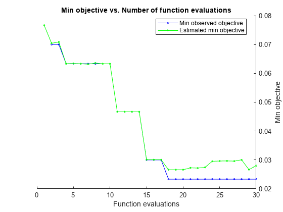
When you call the bayesopt function, specify the objective function as fun and specify the hyperparameters as params_bilayeredNet. Also, specify NumCoupledConstraints as 1 to indicate that the objective function has one coupled constraint. For reproducibility, set the random seed and use the expected-improvement-plus acquisition function.
rng("default")
resultNN = bayesopt(fun,params_bilayeredNet, ...
    AcquisitionFunctionName="expected-improvement-plus", ...
    NumCoupledConstraints=1);
|==================================================================================================================================================|
| Iter | Eval   | Objective   | Objective   | BestSoFar   | BestSoFar   | Constraint1  |  Activations |       Lambda | Layer_1_Size | Layer_2_Size |
|      | result |             | runtime     | (observed)  | (estim.)    |              |              |              |              |              |
|==================================================================================================================================================|
|    1 | Infeas |    0.076667 |      3.8313 |         NaN |    0.076667 |      2.4e+03 |         none |   7.6806e-06 |           15 |          115 |
|    2 | Best   |        0.07 |      1.1425 |        0.07 |    0.070445 |         -196 |         none |    0.0001221 |            2 |            1 |
|    3 | Infeas |     0.46667 |     0.15246 |        0.07 |    0.070862 |     1.39e+03 |      sigmoid |       45.438 |           26 |           14 |
|    4 | Best   |    0.063333 |      1.3051 |    0.063333 |    0.063353 |        -52.5 |         tanh |   2.6069e-05 |            4 |            8 |
|    5 | Accept |     0.11333 |      1.4743 |    0.063333 |    0.063423 |        -58.5 |         relu |   2.2423e-05 |            4 |            7 |
|    6 | Accept |        0.07 |      1.1222 |    0.063333 |    0.063344 |         -196 |         none |    0.0001411 |            2 |            1 |
|    7 | Infeas |    0.046667 |      1.5327 |    0.063333 |     0.06318 |     1.95e+04 |         tanh |   1.2269e-07 |          300 |           16 |
|    8 | Infeas |     0.11333 |       5.227 |    0.063333 |    0.063575 |     9.47e+04 |         tanh |     0.045218 |          298 |          267 |
|    9 | Accept |     0.46667 |    0.023516 |    0.063333 |    0.063332 |         -196 |         none |       9.1357 |            2 |            1 |
|   10 | Infeas |     0.46667 |    0.025527 |    0.063333 |    0.063332 |     1.42e+03 |         relu |       3.0052 |           30 |            7 |
|   11 | Best   |    0.046667 |      2.0311 |    0.046667 |    0.046678 |         -172 |         relu |    6.691e-09 |            2 |            7 |
|   12 | Accept |    0.046667 |      1.0284 |    0.046667 |    0.046675 |        -52.5 |         tanh |   6.7859e-09 |            4 |            8 |
|   13 | Accept |    0.086667 |      2.4386 |    0.046667 |    0.046686 |         -172 |         relu |   1.1251e-07 |            2 |            7 |
|   14 | Accept |     0.46667 |    0.024936 |    0.046667 |     0.04668 |        -58.5 |         tanh |       60.245 |            4 |            7 |
|   15 | Best   |        0.03 |      1.0594 |        0.03 |    0.030086 |        -58.5 |         tanh |    0.0011383 |            4 |            7 |
|   16 | Infeas |     0.12333 |     0.12629 |        0.03 |     0.03007 |          296 |      sigmoid |    6.766e-09 |           10 |            8 |
|   17 | Accept |    0.076667 |     0.71763 |        0.03 |    0.030071 |         -146 |         none |   8.2973e-09 |            3 |            1 |
|   18 | Best   |    0.023333 |      1.0659 |    0.023333 |    0.026599 |        -58.5 |         tanh |    0.0009958 |            4 |            7 |
|   19 | Accept |    0.026667 |        1.01 |    0.023333 |     0.02661 |        -52.5 |         tanh |    0.0009402 |            4 |            8 |
|   20 | Accept |        0.05 |      1.3193 |    0.023333 |    0.026601 |         -226 |      sigmoid |    1.086e-05 |            1 |            8 |
|==================================================================================================================================================|
| Iter | Eval   | Objective   | Objective   | BestSoFar   | BestSoFar   | Constraint1  |  Activations |       Lambda | Layer_1_Size | Layer_2_Size |
|      | result |             | runtime     | (observed)  | (estim.)    |              |              |              |              |              |
|==================================================================================================================================================|
|   21 | Accept |    0.036667 |      1.0198 |    0.023333 |    0.027248 |         -110 |         tanh |   0.00090677 |            3 |            8 |
|   22 | Infeas |    0.053333 |      5.9702 |    0.023333 |    0.027181 |     1.41e+04 |         tanh |   0.00048938 |          283 |            1 |
|   23 | Infeas |     0.12333 |     0.37451 |    0.023333 |    0.027429 |     1.71e+04 |         relu |   7.1367e-09 |          238 |           23 |
|   24 | Accept |    0.076667 |     0.92349 |    0.023333 |    0.029543 |         -248 |         none |   6.7138e-07 |            1 |            1 |
|   25 | Accept |    0.046667 |      1.3113 |    0.023333 |     0.02962 |         -226 |         tanh |   1.1434e-07 |            1 |            8 |
|   26 | Accept |    0.043333 |      1.3654 |    0.023333 |    0.029659 |         -168 |      sigmoid |   9.1787e-07 |            2 |            8 |
|   27 | Accept |    0.043333 |     0.71783 |    0.023333 |    0.029584 |         -226 |         tanh |    0.0018534 |            1 |            8 |
|   28 | Infeas |        0.06 |      3.8672 |    0.023333 |    0.030036 |     1.31e+04 |      sigmoid |   2.3192e-06 |          257 |            2 |
|   29 | Accept |    0.066667 |       1.257 |    0.023333 |    0.026647 |         -226 |         tanh |   0.00050488 |            1 |            8 |
|   30 | Accept |    0.036667 |     0.70965 |    0.023333 |    0.028015 |        -52.5 |         tanh |    0.0044111 |            4 |            8 |
__________________________________________________________
Optimization completed.
MaxObjectiveEvaluations of 30 reached.
Total function evaluations: 30
Total elapsed time: 60.5813 seconds
Total objective function evaluation time: 44.1746

Best observed feasible point:
    Activations     Lambda      Layer_1_Size    Layer_2_Size
    ___________    _________    ____________    ____________

       tanh        0.0009958         4               7

Observed objective function value = 0.023333
Estimated objective function value = 0.029092
Function evaluation time = 1.0659
Observed constraint violations =[ -58.500000 ]

Best estimated feasible point (according to models):
    Activations     Lambda      Layer_1_Size    Layer_2_Size
    ___________    _________    ____________    ____________

       tanh        0.0011383         4               7

Estimated objective function value = 0.028015
Estimated function evaluation time = 1.0464
Estimated constraint violations =[ -58.501089 ]
bayesopt finds optimal hyperparameters that minimize an error in the holdout validation set and satisfy the constraint. Extract the best point in the optimization results resultNN by using the bestPoint function.
[optimalParams,CriterionValue1,iteration] = bestPoint(resultNN)
optimalParams=1×4 table
    Activations     Lambda      Layer_1_Size    Layer_2_Size
    ___________    _________    ____________    ____________

       tanh        0.0011383         4               7
CriterionValue1 = 0.0332
iteration = 15
Train the bilayered neural network model with the optimal hyperparameters.
rng("default")
modelNNOpt = compact(fitcnet(xTrainSelected,yTrainMapped, ...
    Activations=char(optimalParams.Activations), ...
    LayerSizes=[optimalParams.Layer_1_Size optimalParams.Layer_2_Size], ...
    Lambda=optimalParams.Lambda));
Find the accuracy and size of the trained model.
OptimizedNNAccuracy = (1-loss(modelNNOpt,xTestSelected,yTestMapped))*100
OptimizedNNAccuracy = 93.3333
OptimizedNNSize = whos("modelNNOpt").bytes/1024OptimizedNNSize = 8.3555
Quantize Model Parameters with Simulink Block
You can also reduce the memory footprint of a machine learning model by quantizing model parameters with a Simulink® block. Statistics and Machine Learning Toolbox™ provides various prediction blocks that allows you to import a trained machine learning model into a Simulink model. In the prediction blocks, you can specify the data types for some or all model parameters as single-precision, fixed-point, half-precision, and so on. For an example of fixed-point conversion, see Human Activity Recognition Simulink Model for Fixed-Point Deployment.
This example provides the Simulink model slexAcousticSceneClassificationNNPredictExample.slx, which includes the ClassificationNeuralNetwork Predict block. Open this model.
SimMdlName = 'slexAcousticSceneClassificationNNPredictExample';
open_system(SimMdlName)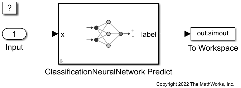
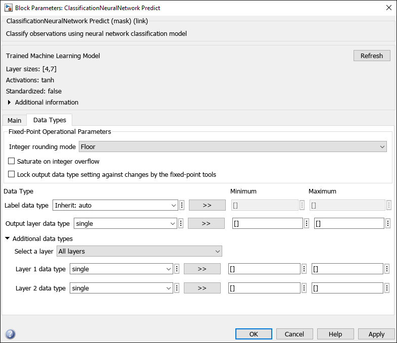
Double-click the ClassificationNeuralNetwork Predict block to open the Block Parameters dialog box. You can specify the data types for the model parameters in the Data Types tab. to reduce the memory size, specify the data types for the layers as single. For details on specifying data types, see Specify Data Types Using Data Type Assistant (Simulink).
Prepare the input data for the Simulink model. Convert the predictor data (xTestSelected) to single precision by using the single function.
soundInput.time = (0:size(xTestSelected,1)-1)';
soundInput.signals(1).values = single(xTestSelected);
soundInput.signals(1).dimensions = size(xTestSelected,2);
Simulate the Simulink model and assign the result to the out variable.
out = sim(SimMdlName);
Find the accuracy of the predict block using the data logged in the To Workspace (Simulink) block.
pred = categorical(out.simout.Data,unique(out.simout.Data),["AllAround","Directional"]);
QuantizedNNAccuracy = sum(pred == yTestMapped)/length(yTestMapped)*100
QuantizedNNAccuracy = 93.3333
Find the size of the quantized model parameters.
p = Simulink.Mask.get("slexAcousticSceneClassificationNNPredictExample/ClassificationNeuralNetwork Predict");
vars = p.getWorkspaceVariables;
blockParams = vars(end).Value;
save("params.mat","blockParams")
s = dir("params.mat");
QuantizedNNSize = s.bytes/1024
QuantizedNNSize = 2.4951
Model Compression Summary
Display the changes in model size and accuracy during the model compression workflow for the bilayered neural network model. In general, the model loses some accuracy as you apply additional model compression schemes.
NNccuracy = [multiMdlTbl{1,"Accuracy"} binaryMdlTbl{1,"Accuracy"} ...
    feat50binaryMdlTbl{1,"Accuracy"} ...
    OptimizedNNAccuracy QuantizedNNAccuracy];
NNSize = [multiMdlTbl{1,"Model Size"} binaryMdlTbl{1,"Model Size"} ...
    feat50binaryMdlTbl{1,"Model Size"} ...
    OptimizedNNSize QuantizedNNSize];
ModelType = ["Multiclass","Binary","50 Features","Optimized","Single Precision"];

figure
yyaxis left
b = bar(NNSize);
xtips = b.XEndPoints;
ytips = b.YEndPoints;
labels = string(round(b.YData,2));
text(xtips,ytips,labels,HorizontalAlignment="center",VerticalAlignment="bottom", ...
    Color='#0072BD')
ylabel("Model Size [KB]")
yyaxis right
plot(NNccuracy,"-o")
ylabel("Accuracy [%]")
xticklabels(ModelType)
grid on
For the bilayered neural network model, the model size decreases to less than 30 KB after you reduce the number of features. The constrained optimization and converting data to single precision further reduce the model size.
The accuracy of the initial multiclass classification model is lower compared to the other models, because the multiclass model classifies sounds into 15 types. After you simplify the multiclass problem into a binary classification problem, the models accurately classify more than 90% of the test data. Reducing the number of features leads to a loss of model accuracy, but the constrained optimization step improves accuracy, and converting data to single precision does not reduce accuracy.
Helper Functions
The helperMdlMetrics function takes a cell array of trained models (Mdls) and test data sets (X and Y) and returns a table of model metrics that includes the model accuracy as a percentage and the model size in KB. The helper function uses the whos function to estimate the model size. However, the size returned by the whos function can be larger than the actual model size required in the generated code for deployment. For example, the generated code does not include information that is not needed for prediction. Consider a CompactClassificationECOC model that uses logistic regression learners. The binary learners in a CompactClassificationECOC model object in the MATLAB® workspace contain the ModelParameters property. However, the model prepared for deployment in the generated code does not contain this property.
function tbl = helperMdlMetrics(Mdls,X,Y)
numMdl = length(Mdls);
metrics = NaN(numMdl,2);
for i = 1 : numMdl
    Mdl = Mdls{i};
    MdlInfo = whos("Mdl");
    metrics(i,:) = [(1-loss(Mdl,X,Y))*100 MdlInfo.bytes/1024];
end
tbl = array2table(metrics, ...
    VariableNames=["Accuracy","Model Size"]);
end
The helperOptimizeConstrainedBilayer function trains a bilayered neural network model using a given set of parameters for the training data, and returns the loss for the holdout validation set. In addition, the function accepts the upper limit (maxSize) for the number of weight parameters in the model and returns a constraint value. A positive constraint value indicates that the number of parameters is greater than the specified limit maxSize.
function [objective,constraint] = helperOptimizeConstrainedBilayer(params,xTrain,yTrain,xEval,yEval,maxSize)
mdl = fitcnet(xTrain,yTrain, ...
    Activations=char(params.Activations), ...
    LayerSizes=[params.Layer_1_Size params.Layer_2_Size], ...
    Lambda=params.Lambda);
objective = loss(mdl,xEval,yEval);

numClasses = size(unique(yTrain),1);
sizeEst = size(xTrain,2)*params.Layer_1_Size + ...
    params.Layer_1_Size*params.Layer_2_Size + ...
    params.Layer_2_Size*numClasses;
constraint = sizeEst - maxSize - 0.5;
end
More About
For constraint-coupled optimization, you can consider minimizing these hyperparameters to limit the memory use, depending on the type of machine learning model:
Decision tree — Minimum number of leaf node observations (MinLeafSize) and the maximum number of decision splits (MaxNumSplits). A decision tree model has a small memory footprint.
Linear discriminant and logistic regression — Number of features and classes. Both a linear discriminant model and a logistic regression model have a small to medium memory footprint.
Shallow neural network — Number of fully connected layers and the number of hidden units in each layer (LayerSizes). A shallow neural network model has a small to medium memory footprint.
k-nearest neighbor — Training data size, the number of nearest neighbors (NumNeighbors), and the maximum number of data points in the leaf node for the Kd-tree algorithm (BucketSize). A k-nearest neighbor model has a medium memory footprint.
Support vector machine (SVM) — Number of support vectors determined by the box constrains (BoxConstraint). An SVM has a medium to large memory footprint. For an SVM model that uses the linear kernel function, you can reduce the footprint by discarding support vectors from the model using the
discardSupportVectorsfunction. The reduced SVM model can still predict new data using predictor coefficients (Betaproperty) stored in the model.Ensemble — Number of learners and the size of each learner determined by NumLearningCycles and Learners. An ensemble has a medium to large memory footprint.
Gaussian process regression (regression only) — Size of the active set (ActiveSetSize). A Gaussian process regression model has a medium to large memory footprint.
Several factors determine the memory use of a machine learning model. However, in general, the memory footprint for a decision tree model is small. A linear discriminant model, logistic regression model, and shallow neural network model have a small to medium memory footprint, and a k-nearest neighbor model has a medium memory footprint. An SVM, ensemble, and Gaussian process model have a medium to large memory footprint. For an SVM model that uses the linear kernel function, you can discard support vectors from the model to reduce the footprint by using the discardSupportVectors function. The reduced SVM model can still predict new data using predictor coefficients (Beta property) stored in the model.
For deployment to memory-limited hardware, a recommended practice is to specify training data using a matrix, not a table. If you specify training data using a table, some model properties, such as PredictorNames, can take a considerable proportion of the model memory footprint.
References
[1] Mesaros, Annamaria, Toni Heittola, and Tuomas Virtanen. Acoustic Scene Classification: An Overview of DCASE 2017 Challenge Entries. In proc. International Workshop on Acoustic Signal Enhancement, 2018.
[2] Lostanlen, Vincent, and Joakim Anden. Binaural Scene Classification with Wavelet Scattering. Technical Report, DCASE2016 Challenge, 2016.
See Also
fscmrmr | bayesopt | discardSupportVectors | ClassificationNeuralNetwork Predict