PWM을 사용한 BLDC 속도 제어를 위한 능동 외란 제거 제어 설계

다음 제품이 필요합니다.

이 예제는 Simscape™ Electrical™ 컴포넌트 사용하여 Simulink®에서 모델링된 BLDC(브러시리스 DC) 모터의 속도에 대한 능동 외란 제거 제어(ADRC)를 설계하는 방법을 보여줍니다.

이 예제에서는 ADRC 제어기와 PID 제어기의 제어 성능도 비교해 봅니다. PID 제어기는 광범위한 동작 범위에서 조정이 가능한 반면 실험 설계와 PID 이득 조정에 상당한 노력이 필요합니다. ADRC를 사용하면 비선형 제어기를 얻을 수 있으며 더 간단한 설정과 적은 조정 노력으로도 더 나은 성능을 달성할 수 있습니다.

BLDC 모터 모델

BLDC 모터는 효율성이 높고 유지관리 비용이 낮다는 측면 등에서 브러시 모터보다 장점이 많습니다. 이 BLDC 모터의 속도는 PWM 제어를 구현하여 제어됩니다. 모터 속도 제어를 위해, 펄스 폭 변조(PWM)를 사용하여 이상적인 DC 전압원을 변조하고 3상 인버터를 통해 공급하여 BLDC 모터를 구동합니다. 이 모델은 PWM을 사용한 BLDC 속도 제어 비디오에서 설명한 모델을 기반으로 합니다.

mdl = 'BLDCMotorADRC';
open_system(mdl)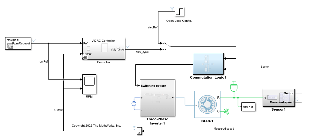

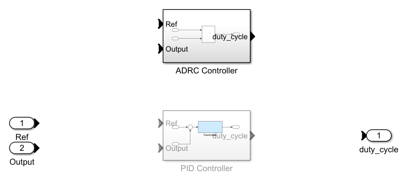
이 모델에는 ADRC 제어기와 PID 제어기 중에서 선택할 수 있는 제어기 Variant Subsystem이 포함되어 있습니다. ADRC Controller 서브시스템이 디폴트 활성 Variant로 설정되어 있습니다. 이 모델에는 모델을 개루프 구성과 폐루프 구성에서 동작시키기 위한 수동 스위치도 포함되어 있습니다. 기본적으로 개루프 구성으로 설정되어 있습니다.

이 모델은 상 전압을 직접 변조하는 방식으로 PWM 제어를 구현합니다. PWM Generator 블록은 Commutation Logic 서브시스템 내에서 사용됩니다. 이 논리에 따라 PWM Generator 블록의 출력은 500V 펄스의 DC 전원 전압을 켜고 꺼서 회전자가 위치한 섹터를 기준으로 올바른 상에 에너지가 주입되도록 합니다.

ADRC 제어기 설계

ADRC는 동특성과 내부 외란, 외부 외란을 알 수 없는 플랜트의 제어기 설계에 사용할 수 있는 강력한 툴입니다. 이 블록은 알 수 없는 동특성과 외란을 플랜트의 확장 상태로 모델링하고 관측기를 사용하여 추정합니다. 이 블록을 사용하면 제어 알고리즘의 몇 가지 핵심적인 조정 파라미터만 사용하여 제어기를 설계할 수 있습니다.

모델 차수 유형(1차 또는 2차)
모델 응답의 임계 이득
제어기와 관측기의 대역폭

또한, 플랜트 모델의 시간 영역과 일치하도록 시간 영역 파라미터를 지정합니다. 이 예제에서는 이산시간으로 설정되어 있으며 샘플 시간은 모델과 함께 제공된 Ts_motor 변수와 같습니다. 다음 섹션에서는 이 모델의 ADRC 블록 파라미터에 지정된 나머지 조정 파라미터를 찾는 방법을 설명합니다.

모델 차수와 임계 이득

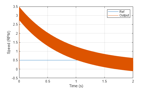
모델 차수를 식별하기 위해 플랜트 모델을 개루프 구성에서 시뮬레이션합니다. 듀티 사이클의 포화 한도가 0부터 1이라고 가정하고, 계단 입력 0.5를 듀티 사이클로 사용하여 플랜트 모델을 구동합니다.

set_param(mdl,'SignalLoggingName','openLoopSim');
sim(mdl);
stepRef = getElement(openLoopSim,'stepRef');
speedOut = getElement(openLoopSim,'Measured speed');
figure;
plot(stepRef.Values.Time,stepRef.Values.Data...
    ,speedOut.Values.Time,speedOut.Values.Data)
grid on
xlabel('Time (s)')
ylabel('Speed (RPM)')
legend('Ref','Output')

Figure contains an axes object. The axes object with xlabel Time (s), ylabel Speed (RPM) contains 2 objects of type line. These objects represent Ref, Output.

임계 이득 값 b0을 결정하기 위해, 스텝 기준 입력 직후 0.00075초의 짧은 간격 동안의 속도 응답을 조사합니다.

x = speedOut.Values.Time(1:16);
y = speedOut.Values.Data(1:16);
figure
plot(x,y)
xlabel('Time (s)')
ylabel('Speed(RPM)')
grid on

Figure contains an axes object. The axes object with xlabel Time (s), ylabel Speed(RPM) contains an object of type line.

y(end)

ans = 
3.1542

속도 응답이 전형적인 2차 동적 시스템의 형태를 보입니다. 따라서 모델 유형 파라미터를 2차로 선택합니다. 측정된 속도를 기반으로 2차 응답 근사 $y = \frac{1}{2} a t^{2}$ 를 통해 임계 이득을 결정할 수 있습니다. 0.0005초 동안 속도가 3.1542rpm만큼 변합니다.

$a = \frac{2 y}{t^{2}}$

$b_{0} = \frac{a}{u}$

a = 2*y(end)/(x(end)^2);
b0 = a/0.5;

제어기 대역폭과 관측기 대역폭

제어기 대역폭은 일반적으로 주파수 영역이나 시간 영역에서의 성능 사양에 따라 달라집니다. 이 예제에서 제어기 대역폭 $ω_{c}$ 는 1000rad/s로 설정되어 있습니다.

일반적으로 관측기 대역폭 $ω_{o}$ 를 $ω_{c}$ 의 5~10배로 설정하여 관측기가 제어기보다 더 빠르게 수렴되도록 합니다. 이 예제에서는 관측기 대역폭을 제어기 대역폭과 동일하게 지정합니다. 이렇게 하면 관측기를 활용하여 PWM으로 제어되는 BLDC 모터에 존재하는 과도한 스위칭 잡음을 필터링할 수 있습니다. 다음 그림은 관측기 대역폭이 1000rad/s와 5000rad/s로 설정되었을 때의 ADRC 제어기 출력 듀티 사이클 신호를 보여줍니다.

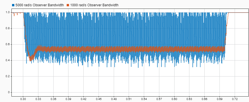
관측기 대역폭이 1000rad/s일 때가 5000rad/s일 때보다 ADRC 블록의 출력 신호의 잡음이 훨씬 적은 것을 확인할 수 있습니다. 현실의 시스템에서는 듀티 사이클 출력이 이처럼 잡음이 많으면 제어기가 사용 불가능해집니다.

관측기 대역폭을 줄이면 ADRC 블록에서 출력 신호의 진동이 줄겠지만, 관측기의 수렴이 느려지면 전반적인 제어 성능에 부정적인 영향을 줄 수 있으므로 $ω_{o}$ 를 더 줄이는 것은 불가능할 수 있습니다.

ADRC 제어기와 PID 제어기의 성능 비교

속도 기준 신호를 변화시키면서 시뮬레이션하면 조정된 제어기의 성능을 검토할 수 있습니다.

제어기의 동적 성능을 검토하기 위해 모델은 다음과 같은 가속 과정을 거칩니다.

t = 0.2초와 t = 0.3초 사이에 속도 기준을 0rpm에서 500rpm까지 올립니다.
t = 0.7초와 t = 1.0초 사이에 속도 기준을 500rpm에서 2000rpm까지 올립니다.

모델이 폐루프 구성에서 동작하도록 수동 스위치를 전환합니다.

set_param('BLDCMotorADRC/Manual Switch','sw','0')

ADRC Controller 서브시스템을 사용하여 모델을 시뮬레이션합니다.

set_param(mdl,'SignalLoggingName','adrcSim');
sim(mdl);
speedOutADRC = getElement(adrcSim,'Measured speed');

PID Controller 서브시스템으로 사용하여 모델을 시뮬레이션합니다.

set_param([mdl,'/Controller'],'LabelModeActiveChoice','PID')
set_param(mdl,'SignalLoggingName','pidSim');
sim(mdl);
speedOutPID = getElement(pidSim,'Measured speed');

두 제어기의 성능을 비교합니다.

figure;
plot(refSignal{1}.Time,refSignal{1}.Data...
    ,speedOutADRC.Values.Time,speedOutADRC.Values.Data)
hold on
plot(speedOutPID.Values.Time,speedOutPID.Values.Data)
hold off
grid on
xlabel('Time (s)')
ylabel('Speed (RPM)')
legend('Ref','ADRC','PID','location','best')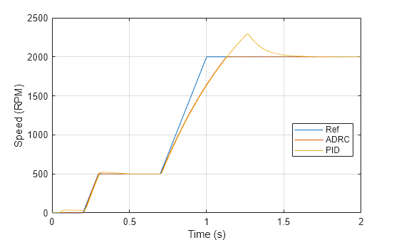

Figure contains an axes object. The axes object with xlabel Time (s), ylabel Speed (RPM) contains 3 objects of type line. These objects represent Ref, ADRC, PID.

속도 응답을 보면 ADRC 제어기가 과도 상태에서 속도 기준을 더 가깝게 추종하고 약 2000rpm에서 오버슈트를 줄임으로써 PID 제어기보다 훨씬 나은 성능을 나타냅니다.

모델을 닫습니다.

close_system(mdl,0);

참고 항목

Active Disturbance Rejection Control