Find Important Parameters for Receptor Occupancy with Global Sensitivity Analysis Using SimBiology Model Analyzer

This example shows how to identify important parameters in a target-mediated drug disposition (TMDD) model [1] using the Global Sensitivity Analysis (GSA) program in SimBiology Model Analyzer. In this example, you compute Sobol indices and elementary effects, and also perform multiparametric GSA (MPGSA) to find model parameters that the target or receptor occupancy (TO) is sensitive to. For more information on supported sensitivity analysis features, see Sensitivity Analysis in SimBiology. The GSA program requires Statistics and Machine Learning Toolbox™.

Target-Mediated Drug Disposition (TMDD) Model

Target-mediated drug disposition (TMDD) is a phenomenon in which a drug binds with high affinity to its pharmacologic target site, such as a receptor or enzyme, in an interaction that is reflected in the pharmacokinetic characteristics of the drug.

This example uses a modified TMDD model based on the model used by Mager and Jusko [1] with a minor adjustment. The authors proposed a generic TMDD model that accounted for saturable drug-target binding and target (or receptor) mediated elimination. Drug in the Plasma reversibly binds with the unbound Target to form the drug-target Complex. kon and koff are the association and dissociation rate constants, respectively. Clearance of free Drug and Complex from the Plasma is described by first-order processes with rate constants — kel and km, respectively. Free target turnover is described by the zero-order synthesis rate ksyn and a first-order elimination (the rate constant, kdeg). Variants of the TMDD model have been since used to characterize the pharmacokinetics of numerous drugs.

One adjustment made to the model presented by Mager and Jusko, is as follows.

Target occupancy (TO) is defined as TO = Complex/(Target + Complex), where TO is a parameter and Complex and Target are species.

Load TMDD Model

Enter the following command. SimBIology Model Analyzer opens. In the Browser pane, the Models folder contains the TMDD model.

openExample('simbio/GSASimBiologyModelAnalyzerExample')

Perform Parameter Scan to Assess Model Behavior

Before performing the global sensitivity analysis on the model, run a parameter scan to get a general idea of how the model response (TO) behaves with respect to parameters of interest. For this example, scan the following model parameters: km, kdeg, and kon.

Select Program > Run Scan. Go to the Generate Samples step of the program. Disable auto plot generation by clicking the plot icon.

In the Parameter Set table, double-click the empty cell in the Component Name column. Enter km. Change Type, Spacing, Min, Max, and # Of Steps options as shown next.

Set up kdeg and kon similarly to km, except use 0.5 as the Max value.

Change Parameter Combination to cartesian. For details about the combination methods, see Combine Simulation Scenarios in SimBiology.

Click Simulation Settings on the Home tab of the app. In the Simulation Time section, change StopTime to 2. In the States To Log section, click Clear All. Then select TO only. Click Close.

Click Run on the Home tab. The program then opens the Plot1 tab. Click Time in the Property Editor pane on the right to see the time courses of the model response (TO) with respect to different parameter combinations of km, kdeg, and kon.

Categorize the plot to make it easier to identify the sources of sensitivity. In the Property Editor pane, under Visual Channels, change the style of km, kdeg, and kon as in the following figure. You need to also change the style of Scenarios from Color to empty.

Click Plot Settings and click Link Y-Axis to use the same Y-axis limit for all plots and to make the plots more comparable. The plot indicates that TO is sensitive to changes in kon and km values. It seems to be less sensitive to variations in kdeg. Optionally, you can also scan one parameter at a time by disabling and enabling the parameters in the Parameter Set table to see the effect of each parameter.

Follow the next steps to perform GSA on these parameters to get more insights into relative contributions of individual parameters that contribute most to the overall model behavior.

Compute Sobol Indices

The section shows you how to perform GSA by computing the first-order and total-order Sobol Indices of model parameters using the Global Sensitivity Analysis program.

Select Program > Global Sensitivity Analysis. By default, the program uses Sobol indices as a GSA analysis method.

Define the model parameters of interest in the Sensitivity Inputs table. Double-click the empty cell under Component Name column and enter km.

By default, the program uses the uniform distribution to sample parameter values. To see a list of supported distributions, click Uniform. For this example, use the uniform distribution and set the Lower and Upper bounds to 1e-3 and 0.1, respectively.

Similarly, set up kdeg and kon as sensitivity inputs. Use 0.5 as the Upper value.

In Sampling Options, use the default values.

Tip: Sampling Types

SimBiology provides the following sampling methods.

• sobol — Use the low-discrepancy Sobol sequence to generate samples. For details, see sobolset (Statistics and Machine Learning Toolbox).

• halton — Use the low-discrepancy Halton sequence to generate samples. For details, see haltonset (Statistics and Machine Learning Toolbox).

• latin hypercube — Use low-discrepancy Latin hypercube samples. If UseLhsDesign is also set to true, SimBiology uses lhsdesign (Statistics and Machine Learning Toolbox). Otherwise, it uses a nonconfigurable Latin hypercube sampler that is different from lhsdesign.

• random — Use randomly distributed samples.

In the Sensitivity Outputs table, enter TO.

Click the Run button of the Sobol Indices step.

The status bar at the bottom of the program provides the run progress and the number of runs that have been finished.

Tip: Total Number of Runs

The total number of runs required is different depending on the number of sensitivity inputs, number of samples, and the GSA analysis method.

• For Sobol Indices, the total number of runs is: (number of sensitivity inputs + 2) ⁢⁢✕ number of samples.

• For Elementary Effects, the total number of runs is: (number of sensitivity inputs + 1) ✕ number of samples.

• For MPGSA, the total number of runs is equal to the number of samples.

The program opens the Datasheet1 and Plot2 tabs. By default, Plot2 shows the GSA Time plot of the first-order and total-order Sobol indices for each input parameter.

The first-order Sobol index of an input parameter gives the fraction of the overall response variance that can be attributed to variations in the input parameter alone. The total-order index gives the fraction of the overall response variance that can be attributed to any joint parameter variations that include variations of the input parameter. Based on the first-order and total-order plots, both km and kon seem to be the sensitive parameters to TO. km seems to become more sensitive at later time points while kon is more sensitive before time = 1. The fraction of unexplained variance plot is a flat line, which means that there is almost no unexplained variance and most variances are accounted for in the first-order and total-order plots.

Tip: Unexplained Variance and Total Variance

The fraction of unexplained variance is calculated as 1 - (sum of all the first-order Sobol indices), and the total variance is calculated using var(response), where response is the model response at every time point.

Tip: Bar Plot

You can also see the bar plot of the Sobol indices by clicking Bar in Plot Settings. The color shading of each bar is a histogram representing values at different times. Darker colors mean that those values occur more often over the whole time course. This plot is especially useful to visualize the Sobol indices of scalar responses or observables.

Click the Datasheet1 tab to view the tables of GSA program results. The first table shows the time dependent responses of Sobol indices. In the second table, you can find out if any model simulation failed during the computation by checking the Number of Successful Samples row. In this example, there were no failed simulations as all 1000 samples were successfully simulated.

Compute Elementary Effects

The following steps show you how to reuse the same program setup in the previous step to compute the means and standard deviations of the Elementary Effects of input parameters with respect to the model response TO.

Given that computing GSA results is often computationally expensive, save the previous Sobol indices results before switching over to elementary effects. In the Browser panel, expand Program2. Right-click LastRun and select Save Data. Enter the name of the data as sobol_results. Click OK.

Tip: Check Project Size

As you save more GSA results, the project size increases. To check the sizes of results from each program and other file contents, open the Project tab by double-clicking the Project icon in the Browser. For details, see Check Saved Models and Data of Project.

Go back to the Program2 tab. In the Sobol Indices step, under the Analysis section, select Sobol indices > Elementary effects.

The Sensitivity Inputs table is automatically set up with the same set of parameters and their corresponding upper and lower bounds as the previous step.

TO is the only sensitivity output. Use the default values for Grid Settings. Click the info icon to display additional information for each option. For details about how the algorithm uses these settings, see Elementary Effects for Global Sensitivity Analysis.

Use the default value (AbsoluteEffects = true) for the Output Settings as well. The program uses the absolute elementary effects by default because the elementary effects can average out when you calculate the mean otherwise.

Click the Run button of the Elementary Effects step. The program then opens the Datasheet2 and Plot3 tabs. By default, Plot3 shows the GSA Time plot of the mean and standard deviation of elementary effects for each input parameter.

The mean of elementary effects explains whether variations in input parameter values have any effect on the model response TO. The mean plots indicate km becomes more sensitive at later time points and kon is more sensitive before time = 0.5. This trend is similar to the Sobol GSA results as well. kdeg also shows some sensitivity but might be insignificant because mean values are much smaller than those of km and kon. The standard deviation of effects explains whether the sensitivity change is dependent on the location in the parameter domain. For instance, the km standard deviation plot indicates larger deviations for larger parameter values in the later stage (time > 0.5).

Tip: Param Grid Plot

Click Param Grid in Plot Settings to visualize the parameter grids and samples used to compute the elementary effects. The grid plot provides a visual of if there was a good coverage over the parameter domain. For this example, there was good coverage as shown in the following figure. For details on how the grid points are selected, see Elementary Effects for Global Sensitivity Analysis.

Tip: Bar Plot

You can also see the bar plot of the means and standard deviations of elementary effects by clicking Bar in Plot Settings. The color shading of each bar is a histogram representing values at different times. Darker colors mean that those values occur more often over the whole time course.

Click the Datasheet2 tab to view the tables of GSA program results. The first table shows the time dependent responses of elementary effects. In the second table, you can find out if any model simulation failed during the computation by checking the Number of Successful Samples row. In this example, there were no failed simulations as all 1000 samples were successfully simulated.

Perform Multiparametric GSA (MPGSA)

The following steps show you how to reuse the same program set up in the previous step to perform Multiparametric GSA (MPGSA) to answer the question of whether the input parameters have any effects on the exposure (area under the curve of the TO profile) threshold for the target occupancy.

Save the previous elementary effects GSA results before switching over to MPGSA. In the Browser panel, expand Program2. Right-click LastRun and select Save Data. Enter the name of the data as ee_results. Click OK.

Click the Program2 tab. In the Elementary Effects step, under the Analysis section, select MPGSA (multi-parametric global sensitivity analysis).

The stop time is set to 2 and the Sensitivity Inputs table is automatically set up with the same number of samples (1000) and the same set of parameters, with their corresponding upper and lower bounds as the previous GSA analysis.

Use default settings for Sampling Options and Correlation Matrix.

In the Classifiers table, double-click the empty cell in the Expression column and enter: trapz(time,TO) <= 0.5. This expression defines an exposure (area under the curve of the TO profile) threshold for the target occupancy. Use the default value (0.05) for Significance Level.

Click the Run button of the MPGSA step. You might see a warning about dimensional analysis not being able to perform. For the purposes of this example, you can ignore the warning.

Tip: The GSA program enables you to perform MPGSA as a standalone analysis or as an added step following the Sobol Indices or Elementary Effects analysis. A benefit of adding MPGSA as a subsequent step is that it can reuse the simulation results from the previous step if possible and saves computation time. To add MPGSA as a subsequent step, click the green plus icon at the top of the GSA program and click MPGSA. The MPGSA subsequent step reuses the simulation results whenever the model response (such as TO) defined in the classifier was used as the sensitivity output in the previous step.

The program then opens Datasheet3 with GSA results and Plot4 showing the bar plot of the MPGSA results for each input parameter. To see the empirical cumulative distribution functions (eCDFs) curves of the results, click eCDF in Plot Settings.

For each parameter, two curves show eCDFs of the accepted and rejected samples. Except for km, the other two parameters do not seem to show a significance difference between the two curves. These plots qualitatively show that km and kon affect the classification of samples while kdeg does not. Quantitatively, the maximum absolute distance between two eCDFs curves is called the Kolmogorov-Smirnov (K-S) distance. The km plot shows a large K-S distance.

To compute the K-S distance between the two eCDFs, SimBiology uses a two-sided test based on the null hypothesis that the two distributions of accepted and rejected samples are equal. See kstest2 (Statistics and Machine Learning Toolbox) for details. If the K-S distance is large, then the two distributions are different, meaning that the classification of the samples is sensitive to variations in the input parameter. On the other hand, if the K-S distance is small, then variations in the input parameter do not affect the classification of samples.

To assess the significance of the K-S statistic rejecting the null-hypothesis, you can examine the p-values by looking at the bar plot. Click Bar in the Plot Settings.

The bar plot shows two bars for each parameter: one for the K-S distance (K-S statistic) and another for the corresponding p-value. You reject the null hypothesis if the p-value is less than the significance level. A cross (x) is shown for any p-value that is almost 0.

The p-values for km and kon are less than the significance level (0.05), supporting the alternative hypothesis that the accepted and rejected samples come from different distributions. The p-value of kdeg is larger than the significance level supporting the null hypothesis that the accepted and rejected samples come from the same distribution. To conclude, the classification of the samples is sensitive to km and kon, not kdeg. These results are in agreement with the previous GSA results which identify km and kon as sensitive parameters but not kdeg.

To see the exact p-value corresponding to each parameter, click Datasheet3.

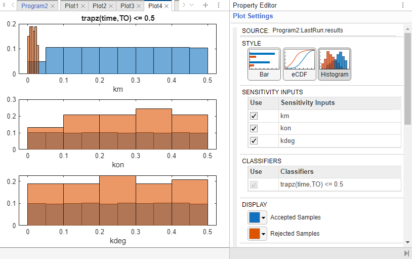
Tip: Histogram of Accepted and Rejected Samples

You can also check the histogram of accepted and rejected samples to see if there are any trends. Click the Plot4 tab. Click Histogram in the Plot Settings. The histogram of km shows that km is primarily responsible for the sensitivity of the AUC being less than the threshold 0.5.

References

[1] Marger, D., and W. Jusko. 2001. General pharmacokinetic model for drugs exhibiting target-mediated drug disposition. Journal of Pharmacokinetics and Pharmacodynamics. 28: 507–532.