Analytic Signal for Cosine
This example shows how to determine the analytic signal. The example also demonstrates that the imaginary part of the analytic signal corresponding to a cosine is a sine with the same frequency. If the cosine has a nonzero mean (DC shift), then the real part of the analytic signal is the original cosine with the same mean, but the imaginary part has zero mean.
Create a cosine with a frequency of 100 Hz. The sample rate is 10 kHz. Add a DC offset of 2.5 to the cosine.
t = 0:1e-4:1;
x = 2.5 + cos(2*pi*100*t);
Use the hilbert function to obtain the analytic signal. The real part is equal to the original signal. The imaginary part is the Hilbert transform of the original signal. Plot the real and imaginary parts for comparison.
y = hilbert(x);

plot(t,real(y))
hold on
plot(t,imag(y))
xlim([0 0.1])
grid on
text([0.015 0.015],[3.7 1.2], ...
    {'Real Part \downarrow';'Imaginary Part \downarrow'})
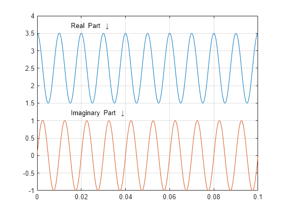
You see that the imaginary part is a sine with the same frequency as the cosine real part. However, the imaginary part has a mean of zero, while the real part has a mean of 2.5.
The original signal is
The resulting analytic signal is
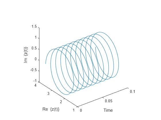
Plot 10 periods of the complex-valued analytic signal.
prds = 1:1000;

figure
plot3(t(prds),real(y(prds)),imag(y(prds)))

xlabel('Time')
ylabel('Re \{z(t)\}')
zlabel('Im \{z(t)\}')
axis square