refinepeaks
Syntax
Description
[
refines peaks based on a signal with amplitudes yRPeaks,xRPeaks] = refinepeaks(y,xPeaksIdx)y, and indices of the
initial peak estimates xPeaksIdx, returning the refined peak values
yRPeaks and location estimates xRPeaks. This
syntax uses quadratic least squares processing to refine the peaks based on
xRPeaks and two surrounding points for every selected peak.
[___] = refinepeaks(___,
specifies additional options, such as the peak refinement method and method specifications,
using name-value arguments. Use this syntax with any of the input or output arguments in
preceding syntaxes.Name=Value)
refinepeaks(___) with no output arguments draws a
figure that compares the refined peak amplitudes and locations to the initial peak estimates
and their surrounding samples. The figure also plots the fitting curves used to refine the
peaks. The refinepeaks function plots the three-point sets with
unfilled circles and plots the refined peaks with filled circles.
Examples
Refine a known peak from a signal specified as a vector or as a MATLAB® timetable.
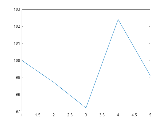
Create a five-element vector. Set the fourth sample so that it is a local maximum. Plot the function and observe that the fourth sample is a signal peak with an amplitude of 102.4.
Intensity = [100;98.7;97.2;102.4;99.1];
plot(Intensity)
Refine the known peak and compute its refined value and location. The refined peak is located slightly after the original peak on the fourth sample of the signal.
[YRpeak,XRpeak] = refinepeaks(Intensity,4)
YRpeak =
102.4531
XRpeak =
4.1118
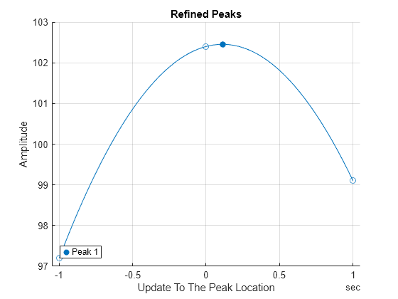
Create a timetable from a signal, using a sample rate of 1 Hz.
TT = timetable(Intensity,SampleRate=1)
TT=5×1 timetable
    Time     Intensity
    _____    _________

    0 sec        100
    1 sec       98.7
    2 sec       97.2
    3 sec      102.4
    4 sec       99.1
Refine the peak and plot the result. Observe that the refined peak occurs 0.11 seconds after the initial estimate, and the refined peak value of 102.45 shows as a filled circle. The original peak is at 0 seconds for reference, while the surrounding points are at -1 second and 1 second from the reference.
refinepeaks(TT,4)
Generate a Rayleigh distribution with a scale parameter b set to .
P = @(x,b) (x/b^2).*exp(-0.5*(x/b).^2);
x = 0:2.5:20;
b = pi;
p = P(x,b);
plot(x,p)
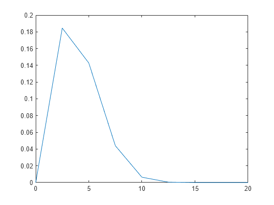
Calculate the theoretical and estimated peak amplitude and location. The peak is located about half of a sample from the expected peak scaled location, .
yPeakTheo = P(b,b);
xPeakTheo = b;
yPeakEst = max(p);
xPeakIdx = find(p==max(p));
xPeakEst = x(xPeakIdx);
disp(table(["Estimated";"Theoretical"], ...
    [yPeakEst;yPeakTheo],[xPeakEst;xPeakTheo], ...
    VariableNames=["Peak" "Amplitude" "Location"]))
        Peak         Amplitude    Location
    _____________    _________    ________

    "Estimated"       0.18456         2.5
    "Theoretical"     0.19306      3.1416
Refine the peak estimation using the quadratic least squares (QLS) method with default specifications.
[yRPeakDef,xRPeakDef] = refinepeaks(p,xPeakIdx,x);
Refine the peak estimation using the QLS method by specifying an exponential kernel with an exponent value of three.
[yPeakRef,xPeakRef] = refinepeaks(p,xPeakIdx,x, ...
    Method="QLS",QLSKernel="exp",KernelPower=3);
Compare the peak refinement results. The refined peak amplitude and location with both QLS-method variants yield a better approximation of the theoretical values than do the initial estimates. The exponential kernel yields the best approximation of the peak theoretical values for the specified Rayleigh distribution.
disp(table(["Initial Estimation";"Refined (QLS default)"; ...
    "Refined (QLS customized)";"Theoretical"], ...
    [yPeakEst;yRPeakDef;yPeakRef;yPeakTheo], ...
    [xPeakEst;xRPeakDef;xPeakRef;xPeakTheo], ...
    VariableNames=["Peak" "Amplitude" "Location"]))
               Peak               Amplitude    Location
    __________________________    _________    ________

    "Initial Estimation"           0.18456         2.5
    "Refined (QLS default)"        0.19581      3.2884
    "Refined (QLS customized)"     0.19315      3.2398
    "Theoretical"                  0.19306      3.1416
Obtain a refined peak location estimate for the main two peaks in a signal using the nonlinear least squares method with a sinc function kernel.
Generate Signal
Radar pulse compression of a linear FM waveform produces a sinc-shaped spectrum, where the frequency locations of the peaks are proportional to the distance between the radar and the detected object. You can first estimate the peak locations and amplitudes with findpeaks and then enhance your estimates with refinepeaks. This example finds the peak amplitudes and locations of a synthetic noiseless pulse compression signal and uses refinepeaks to improve the estimates.
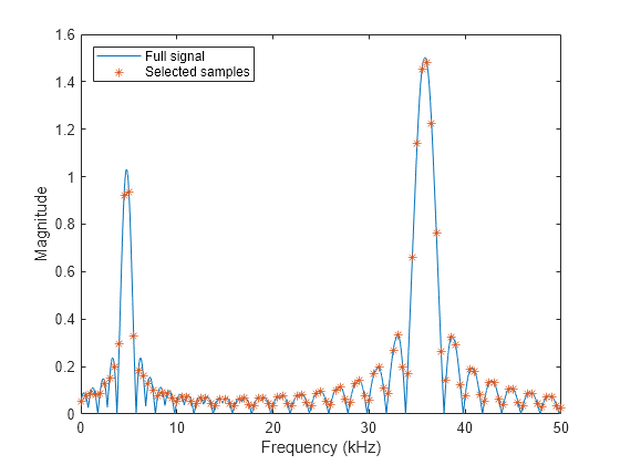
Generate a signal composed of two sinc-shaped waveforms with peaks of 1 and 1.5 at 4.76 kHz and 35.8 kHz, respectively. Set the frequency spacing to 2.5 Hz.
aTg = [1 1.5];
fTg = 1e3*[4.76 35.8];
freqkHzFull = (0:0.0025:50)';
waveFull = abs(sinc([1 0.5].*(freqkHzFull-fTg/1e3)))*aTg';
Downsample the signal by a factor of 200 so the frequency spacing between samples is 0.5 kHz. This example refines the amplitude and location estimates of the downsampled signal peaks and compares the improved estimates to the values in the original signals.
freq = downsample(freqkHzFull,200);
wave = downsample(waveFull,200);

plot(freqkHzFull,waveFull,freq,wave,"*")
legend(["Full signal" "Selected samples"],Location="northwest")
xlabel("Frequency (kHz)")
ylabel("Magnitude")
Refine Peaks Using Nonlinear Least Squares
Use findpeaks to make initial estimates of the amplitudes, locations, and half-height widths of the two highest peaks of the signal.
[PV,PL,PW] = findpeaks(wave,NPeaks=2, ...
    SortStr="descend",WidthReference="halfheight");
table(PV,freq(PL), RowNames="Peak estimate "+(1:numel(PV)), ...
    VariableNames=["Amplitude" "Frequency (kHz)"])
ans=2×2 table
                       Amplitude    Frequency (kHz)
                       _________    _______________

    Peak estimate 1     1.4824            36
    Peak estimate 2     0.9374             5
Use refinepeaks to enhance the peak estimation using the nonlinear least squares (NLS) method. Specify the frequency points of the signal and the peak widths. The peak values are significantly closer to the expected values of 1.5 and 1, while the frequency locations approximate well to 35.8 kHz and 4.76 kHz, respectively.
LW = max(PW,2);
[Ypk,Xpk] = refinepeaks(wave,PL,freq,Method="NLS",LobeWidth=LW);
table(Ypk,Xpk, RowNames="Refined peak "+(1:numel(Ypk)), ...
    VariableNames=["Amplitude" "Frequency (kHz)"])
ans=2×2 table
                      Amplitude    Frequency (kHz)
                      _________    _______________

    Refined peak 1     1.5063            35.8
    Refined peak 2     1.0163          4.7628
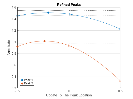
Plot the amplitudes of the refined peaks on the y-axis and the updated peak locations compared with the initial peak estimates on the x-axis. The two initially estimated peaks and their two surrounding samples are each separated by 0.5 kHz. The refined peaks, indicated by filled circles, show the actual peak locations compared to the initially estimated peak locations as well as the corrected amplitudes.
refinepeaks(wave,PL,freq,Method="NLS",LobeWidth=LW)
yline(aTg) % Theoretical peak amplitudes
errorBounds = aTg.*(1+0.03*[-1;1]);
yline(errorBounds(:),":") % ±3% error bounds
legend("Peak "+[1 2])
Identify and refine peaks from hourly temperature data across rows, columns, and pages.
Plot Data
Load a MAT file containing a set of temperature readings in degrees Celsius taken every hour at Boston Logan International Airport for the entire month of January 2011.
load bostemp
tempArray = (tempC(1:24*28))';
timeArray = 1 + (0:numel(tempArray)-1)/24;
Reshape the data from the first 28 days into a three-dimensional array with 24 rows (hours of the day), 7 columns (weekdays), and 4 pages (weeks).
temps3D = reshape(tempArray,[24 7 4]);
times3D = reshape(timeArray,[24 7 4]);
Plot the temperatures across weeks.
temps2D = reshape(temps3D,[24*7 4]);
times2D = reshape(times3D,[24*7 4]);
stem3((1:4).*ones(size(times2D)),1+mod(times2D-1,7),temps2D,".")
view([-20 25])
set(gca,Ydir="reverse")
grid on
axis tight
xticks(1:4)
yticks(1:7)
xlabel("Week Number")
ylabel("Weekday")
zlabel("Temperature (\circC)")
Choose Dimension and Peak Index Format
By default, refinepeaks refines the peaks across the first dimension of the input data array that has more than three samples. In this example, the first dimension (rows) of temps3D has a length of 24 samples, so refinepeaks refines the peaks across rows. Optionally, you can specify Dimension=d to refine the peaks across rows (d=1), columns (d=2) or pages (d=3).
Since the input data temps3D is a 3-D array, you can provide the indices of the initial peak estimates either as a three-column matrix containing the indices columns [iPks jPks kPks] with as many rows as peaks, or as a logical matrix of the same size as temps3D, where each true (logical 1) value points to a peak. This example shows how to specify peak indices in both formats.
Peaks Across Hours (Rows)
Find the temperature peaks on the third day of the fourth week. Estimate the peak amplitudes and locations.
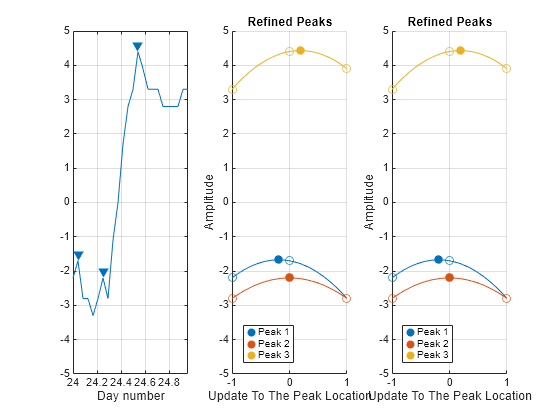
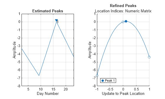
jPks = 3;
kPks = 4;
[EstPks,iPks] = findpeaks(temps3D(:,jPks,kPks));

tiledlayout("horizontal")
ax11 = nexttile;
findpeaks(temps3D(:,jPks,kPks),times3D(:,jPks,kPks))
text(times3D(iPks,jPks,kPks)+0.02,EstPks,string((1:numel(EstPks))'))
xlabel("Day Number")
ylabel("Amplitude")
title("Estimated Peaks")
Specify the indices of the initially estimated peaks as a three-column matrix and refine the peaks across rows. Plot the estimated and refined peaks.
ax12 = nexttile;
xPeaks2D = [0 jPks kPks] + [1 0 0].*iPks;
refinepeaks(temps3D,xPeaks2D)
subtitle(["Location Indices:";"Numeric Matrix"])
Define a logical array specifying a value of true at the indices of the initially estimated peaks. Specify the logical array as the peak location index input to refine the peaks. Plot the refined peaks. Whether you specify the location indices of the initially estimated peaks as a numeric matrix or a logical array, the result is the same.
ax13 = nexttile;
xPeaks3D = false(size(temps3D));
xPeaks3D(iPks,jPks,kPks) = true; % Logical indices
refinepeaks(temps3D,xPeaks3D) % Refined peaks
subtitle(["Location Indices:";"Logical Array"])
linkaxes([ax11 ax12 ax13],"y")
Peaks Across Weekdays (Columns)
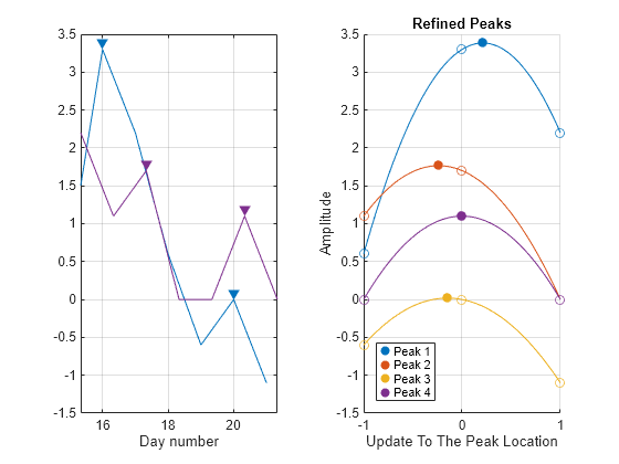
Find the temperature peaks at midnight and at 8 a.m. along all weekdays of the third week. Estimate the peak amplitudes and locations. Specify a logical array of initially estimated peaks and refine the peaks across columns. Plot the estimated and refined peaks.
iPks1 = 1;
iPks2 = 9;
kPks = 3;
[EstPks1,jPks1] = findpeaks(temps3D(iPks1,:,kPks));
[EstPks2,jPks2] = findpeaks(temps3D(iPks2,:,kPks));

tiledlayout("horizontal")
ax21 = nexttile;
findpeaks(temps3D(iPks1,:,kPks),times3D(iPks1,:,kPks))
text(times3D(iPks1,jPks1,kPks)+.02,EstPks1,string((1:numel(EstPks1))'))
hold on
findpeaks(temps3D(iPks2,:,kPks),times3D(iPks2,:,kPks))
text(times3D(iPks2,jPks2,kPks)+.02,EstPks2, ...
    string(numel(EstPks1)+(1:numel(EstPks2))'))
hold off
legend(["12 a.m." "" "8 a.m."])
xlabel("Day Number")
ylabel("Amplitude")
title("Estimated Peaks")

ax22 = nexttile;
xPeaks3D = false(size(temps3D));
xPeaks3D(iPks1,jPks1,kPks) = true;
xPeaks3D(iPks2,jPks2,kPks) = true;
refinepeaks(temps3D,xPeaks3D,Dimension=2)
subtitle("Location Indices: Logical Array")
linkaxes([ax21 ax22],"y")
Peaks Across Weeks (Pages)
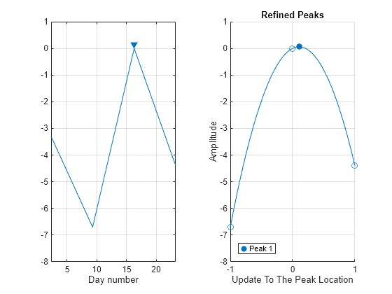
Find the temperature peaks at 7 a.m. during the second day of all weeks. Estimate the peak amplitudes and locations. Specify the indices of the initially estimated peaks as a three-column matrix and refine the peaks across pages. Plot the estimated and refined peaks.
iPks = 8;
jPks = 2;
tempsD27am = temps3D(iPks,jPks,:);
timesD27am = times3D(iPks,jPks,:);
[EstPks,kPks] = findpeaks(tempsD27am(:));

tiledlayout("horizontal")
ax31 = nexttile;
findpeaks(tempsD27am(:),timesD27am(:));
text(times3D(iPks,jPks,kPks)+0.02,EstPks,string((1:numel(EstPks))'))
xlabel("Day Number")
ylabel("Amplitude")
title("Estimated Peaks")

ax32 = nexttile;
xPeaks2D = [iPks jPks 0] + [0 0 1].*kPks;
refinepeaks(temps3D,xPeaks2D,Dimension=3)
subtitle("Location Indices: Numeric Matrix")
linkaxes([ax31 ax32],"y")
Input Arguments
Name-Value Arguments
Output Arguments
Tips
You can initially estimate signal peaks with findpeaks, and then enhance their amplitudes and locations with
refinepeaks.
Assume you have a signal with amplitudes y and locations
x. The following code snippet shows how you can estimate and refine
peaks from y and x.
[yPeaks,xPeaksIdx] = findpeaks(y);
[yRPeaks,xRPeaks] = refinepeaks(y,xPeaksIdx,x)
Add name-value arguments for further customization. For example, you can specify
LobeWidth from the width of the initially estimated
peaks.
[yPeaks,xPeaksIdx,xWidths] = findpeaks(y);
[yRPeaks,xRPeaks] = refinepeaks(y,xPeaksIdx,x,Method="NLS", ...
    LobeWidth=max(xWidths,2))
Algorithms
References
[1] Richards, Mark A., James A. Scheer, and William A. Holm, eds. Principles of Modern Radar: Basic Principles. Institution of Engineering and Technology, 2010.
[2] Moddemeijer, R. “On the Determination of the Position of Extrema of Sampled Correlators.” IEEE® Transactions on Signal Processing 39, no. 1 (January 1991): 216–19.
[3] Sharp, I., K. Yu, and Y. J. Guo. “Peak and Leading Edge Detection for Time-of-Arrival Estimation in Band-Limited Positioning Systems.” IET Communications 3, no. 10 (October 1, 2009): 1616–27.
[4] Prager, Samuel, Mark S. Haynes, and Mahta Moghaddam. “Wireless Subnanosecond RF Synchronization for Distributed Ultrawideband Software-Defined Radar Networks.” IEEE Transactions on Microwave Theory and Techniques 68, no. 11 (November 2020): 4787–4804.
Extended Capabilities
Version History
Introduced in R2024b
See Also
findpeaks | islocalmax | max