instbw

Estimate instantaneous bandwidth

Since R2021a

Syntax

ibw = instbw(x,fs)

ibw = instbw(x,t)

ibw = instbw(xt)

ibw = instbw(tfd,fd,td)

ibw = instbw(___,Name=Value)

[ibw,t] = instbw(___)

instbw(___)

Description

ibw = instbw(x,fs) estimates the instantaneous bandwidth of a signal, x, sampled at a rate fs. If x is a matrix, then the function estimates the instantaneous bandwidth independently for each column and returns the result in the corresponding column of ibw.

ibw = instbw(x,t) estimates the instantaneous bandwidth of x sampled at the time values stored in t.

ibw = instbw(xt) estimates the instantaneous bandwidth of a signal stored in the MATLAB^® timetable xt. The function treats all variables in the timetable and all columns inside each variable independently.

ibw = instbw(tfd,fd,td) estimates the instantaneous bandwidth of the signal whose time-frequency distribution, tfd, is sampled at the bandwidth values stored in fd and the time values stored in td.

ibw = instbw(___,Name=Value) specifies additional options for any of the previous syntaxes using name-value arguments. You can specify the scale factor or the frequency limits used in the computation. For example, FrequencyLimits=[10 20] computes the instantaneous bandwidth of the input in the range from 10 Hz to 20 Hz.

[ibw,t] = instbw(___) also returns t, a vector of sample times corresponding to ibw.

instbw(___) with no output arguments plots the estimated instantaneous bandwidth.

Examples

Instantaneous Bandwidth of Sinusoidal Chirp

Generate a signal sampled at 600 Hz for 2 seconds. The signal consists of a chirp with sinusoidally varying frequency content.

fs = 6e2;

x = vco(sin(2*pi*(0:1/fs:2)),[0.1 0.4]*fs,fs);

Compute the spectrogram of the signal and display it as a waterfall plot.

[p,f,t] = pspectrum(x,fs,'spectrogram');

waterfall(f,t,p')
ax = gca;
ax.XDir = 'reverse';
view(30,45)

Estimate and plot the instantaneous bandwidth of the signal.

instbw(x,fs)
ylim([0 50])

Instantaneous Bandwidth from Spectrogram

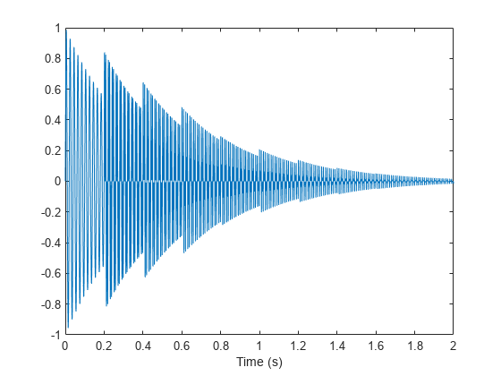
Generate a signal sampled at 2 kHz for 2 seconds. The signal consists of a superposition of exponentially damped sinusoids of increasing frequency that are added at regular intervals. Plot the signal.

fs = 2000;
t = 0:1/fs:2-1/fs;

frq = (50:100:950)';

amp = (t > 4*(frq-frq(1))/fs);
x = sum(amp.*sin(2*pi*t.*frq).*exp(-3*t));

% To hear, type sound(x,fs)

plot(t,x)
xlabel('Time (s)')

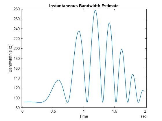
Compute and display the instantaneous bandwidth of the signal.

[bw,bt] = instbw(x,t);

plot(bt,bw)
xlabel('Time (s)')
ylabel('Bandwidth (Hz)')

Compute the spectrogram of the signal. Specify a time resolution of 100 milliseconds and 0 overlap between adjoining segments. Use the spectrogram to estimate the instantaneous frequency of the signal.

[p,ff,tt] = pspectrum(x,t,"spectrogram", ...
    TimeResolution=0.1,OverlapPercent=0);

instfreq(p,ff,tt)

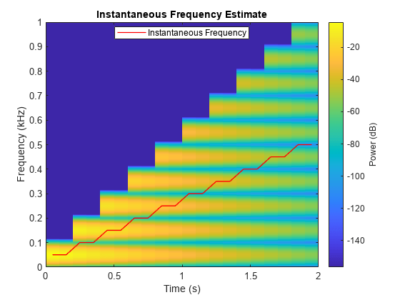
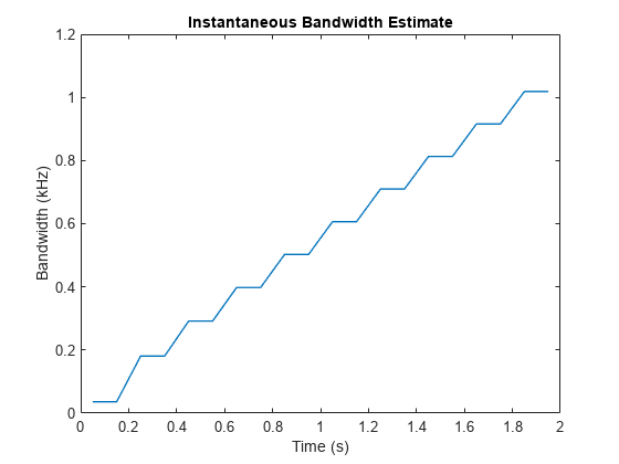
Use the spectrogram to compute the instantaneous bandwidth.

instbw(p,ff,tt)

Instantaneous Bandwidth of Timetable

Generate a signal sampled at 14 kHz for 2 seconds. The frequency of the signal varies as a chirp modulated by a Gaussian. Save the signal as a MATLAB® timetable.

fs = 14000;
t = (0:1/fs:2)';
s = vco(chirp(t+.1,0,t(end),3).*exp(-2*(t-1).^2),[0.1 0.4]*fs,fs);

sx = timetable(s,'SampleRate',fs);

Compute the spectrogram of the signal. Specify a leakage of 0.2, a time resolution of 50 milliseconds, and 99% of overlap between adjoining segments. Display the spectrogram.

opts = {"spectrogram","Leakage",0.2, ...
    "TimeResolution",0.05,"OverlapPercent",99};

[p,ff,tt] = pspectrum(sx,opts{:});

pspectrum(sx,opts{:})

Estimate and display the instantaneous bandwidth of the signal.

instbw(p,ff,tt)

Instantaneous Frequency and Bandwidth as Conditional Spectral Moments

Generate a signal that consists of a chirp whose frequency varies sinusoidally between 300 Hz and 1200 Hz. The signal is sampled at 3 kHz for 2 seconds.

fs = 3e3;
t = 0:1/fs:2;
y = vco(cos(2*pi*t),[0.1 0.4]*fs,fs);

Use instfreq to compute the instantaneous frequency of the signal and the corresponding sample times. Verify that the output corresponds to the noncentralized first-order conditional spectral moment of the time-frequency distribution of the signal as computed by tfsmoment (Predictive Maintenance Toolbox).

[z,tz] = instfreq(y,fs);
[a,ta] = tfsmoment(y,fs,1,Centralize=false);

plot(tz,z,ta,a,".")
legend("instfreq","tfsmoment")

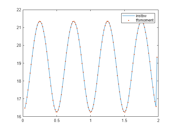
Use instbw to compute the instantaneous bandwidth of the signal and the corresponding sample times. Specify a scale factor of 1. Verify that the output corresponds to the square root of the centralized second-order conditional spectral moment of the time-distribution of the signal. In other words, instbw generates a standard deviation and tfsmoment generates a variance.

[w,tw] = instbw(y,fs,ScaleFactor=1);
[m,tm] = tfsmoment(y,fs,2);

plot(tw,w,tm,sqrt(m),".")
legend("instbw","tfsmoment")

Input Arguments

x — Input signal

vector | matrix

Input signal, specified as a vector or matrix. If x is a vector, then instbw treats it as a single channel. If x is a matrix, then the function computes the instantaneous bandwidth independently for each column and returns the result in the corresponding column of ibw.

Example: sin(2*pi*(0:127)/16)+randn(1,128)/100 specifies a noisy sinusoid.

Example: [2 1].*sin(2*pi*(0:127)'./[16 64]) specifies a two-channel sinusoid.

Data Types: single | double
Complex Number Support: Yes

fs — Sample rate

positive scalar

Sample rate, specified as a positive scalar. The sample rate is the number of samples per unit time. If the unit of time is seconds, then the sample rate is in Hz.

Data Types: single | double | int8 | int16 | int32 | int64 | uint8 | uint16 | uint32 | uint64

t — Sample times

real vector | duration scalar | duration array | datetime array

Sample times, specified as a real vector, a duration scalar, a duration array, or a datetime array.

• duration scalar — The time interval between consecutive samples of x.

• Real vector, duration array, or datetime array — The time instant corresponding to each element of x.

Example: seconds(1) specifies a 1-second lapse between consecutive measurements of a signal.

Example: seconds(0:8) specifies that a signal is sampled at 1 Hz for 8 seconds.

Data Types: single | double | duration | datetime

xt — Input timetable

timetable

Input timetable. xt must contain increasing, finite row times.

If a timetable has missing or duplicate time points, you can fix it using the tips in Clean Timetable with Missing, Duplicate, or Nonuniform Times.

Example: timetable(seconds(0:4)',randn(5,1)) specifies a random process sampled at 1 Hz for 4 seconds.

Example: timetable(seconds(0:4)',randn(5,3),randn(5,4)) contains a three-channel random process and a four-channel random process, both sampled at 1 Hz for 4 seconds.

Data Types: single | double
Complex Number Support: Yes

tfd — Time-frequency distribution

matrix

Time-frequency distribution, specified as a matrix sampled at the frequencies stored in fd and the time values stored in td.

Example: [p,f,t] = pspectrum(sin(2*pi*(0:511)/4),4,"spectrogram") specifies the time-frequency distribution of a 1 Hz sinusoid sampled at 4 Hz for 128 seconds, and also the frequencies and times at which it is computed.

Data Types: single | double

fd, td — Frequency and time values for time-frequency distribution

vectors

Frequency and time values for time-frequency distribution, specified as vectors.

Example: [p,f,t] = pspectrum(sin(2*pi*(0:511)/4),4,"spectrogram") specifies the time-frequency distribution of a 1 Hz sinusoid sampled at 4 Hz for 128 seconds, and also the frequencies and times at which it is computed.

Data Types: single | double

Name-Value Arguments

Specify optional pairs of arguments as Name1=Value1,...,NameN=ValueN, where Name is the argument name and Value is the corresponding value. Name-value arguments must appear after other arguments, but the order of the pairs does not matter.

Before R2021a, use commas to separate each name and value, and enclose Name in quotes.

Example: 'FrequencyLimits',[25 50] computes the instantaneous bandwidth of the input in the range from 25 Hz to 50 Hz.

FrequencyLimits — Frequency range

[0 fs/2] (default for real-valued signals) | [-fs/2 fs/2] (default for complex-valued signals) | two-element vector in Hz

Frequency range, specified as a two-element vector in Hz. If you do not specify FrequencyLimits, then this argument defaults to [0 fs/2] for real-valued signals and to [-fs/2 fs/2] for complex-valued signals.

Data Types: single | double

ScaleFactor — Scaling factor for spectral moment

sqrt(4*pi) (default) | real scalar

Scaling factor for spectral moment, specified as a real scalar.

Data Types: single | double

Output Arguments

ibw — Instantaneous bandwidth

vector | matrix | timetable

Instantaneous bandwidth, returned as a vector, a matrix, or a timetable with the same dimensions as the input.

Data Types: single | double

t — Times of bandwidth estimates

real vector | duration array | datetime array

Times of bandwidth estimates, returned as a real vector, a duration array, or a datetime array.

Data Types: single | double

Note

If t, fd, or td are in single precision and the input vector or matrix is in double precision, then the function returns the output in single precision. The output data type does not depend on the sample rate data type.

More About

Instantaneous Bandwidth

The instantaneous bandwidth of a nonstationary signal is a time-varying parameter that relates to the spread of the instantaneous frequency about its average at a given time instant [1], [2].

instbw estimates the instantaneous bandwidth as the square-root of the second conditional spectral moment of the time-frequency distribution of the input signal. The function:

1. Computes the spectrogram power spectrum P(t,f) of the input using the pspectrum function and uses the spectrum as a time-frequency distribution.

2. Estimates the instantaneous bandwidth using

   $${\sigma }_f{}^2\left(t\right)=\frac{{\displaystyle {\int }_0^{\infty }{\left(f-f_{\text{inst}}\left(t\right)\right)}^{2}P\left(t,f\right)df}}{{\displaystyle {\int }_0^{\infty }P\left(t,f\right)df}},$$

   where $$f_{\text{inst}}\left(t\right)$$ is the instantaneous frequency returned by instfreq and estimated by

   $$f_{\text{inst}}(t)=\frac{{\displaystyle {\int }_0^{\infty }fP(t,f)df}}{{\displaystyle {\int }_0^{\infty }P(t,f)df}}.$$

References

[1] Boashash, Boualem. “Estimating and Interpreting the Instantaneous Frequency of a Signal. I. Fundamentals.” Proceedings of the IEEE^® 80, no. 4 (April 1992): 520–538. https://doi.org/10.1109/5.135376.

[2] Boashash, Boualem. "Estimating and Interpreting The Instantaneous Frequency of a Signal. II. Algorithms and Applications." Proceedings of the IEEE 80, no. 4 (May 1992): 540–568. https://doi.org/10.1109/5.135378.

Extended Capabilities

C/C++ Code Generation
Generate C and C++ code using MATLAB® Coder™.

GPU Arrays

Accelerate code by running on a graphics processing unit (GPU) using Parallel Computing Toolbox™.

This function fully supports GPU arrays. For more information, see Run MATLAB Functions on a GPU (Parallel Computing Toolbox).

Version History

Introduced in R2021a

R2023b: Use timetables for code generation

The instbw function supports MATLAB timetables for code generation.

R2022b: Use gpuArray objects

The instbw function supports gpuArray objects. You must have Parallel Computing Toolbox™ to use this functionality.