Access
Access analysis object belonging to scenario
Description
The Access object defines an access analysis object belonging to a Satellite, GroundStation, ConicalSensor, or Platform object. Use this
object to determine if the line-of-sight (LOS) between two objects exists.
Also,
If one of the objects belongs to
GroundStation, the MinElevationAngle property of theGroundStationobject limits the LOS visibility.If one of the objects belongs to
ConicalSensor, the MaxViewAngle property of theConicalSensorobject limits the LOS visibility.
For more information see, Algorithms.
Note
Access object visibility analysis does not take terrain or building obstructions into account.
Creation
You can create an Access object using the access object function of
Satellite, GroundStation, ConicalSensor, or Platform.
Properties
IDs of the satellites, ground stations, platforms, or conical sensors defining access analysis, specified as a vector of positive numbers.
Obstructing bodies to be considered in LOS access calculations, specified as a
string or string array consisting of "Earth",
"Moon", or ["Earth", "Moon"].
Note
Including Moon as an obstructing body requires an Aerospace Toolbox license.
Visual width of access analysis object in pixels, specified as a scalar in the range (0, 10].
The line width cannot be thinner than the width of a pixel. If you set the line width to a value that is less than the width of a pixel on your system, the line displays as one pixel wide.
Color of access analysis line, specified as an RGB triplet, hexadecimal color code, a color name, or a short name.
For a custom color, specify an RGB triplet or a hexadecimal color code.
An RGB triplet is a three-element row vector whose elements specify the intensities of the red, green, and blue components of the color. The intensities must be in the range
[0,1], for example,[0.4 0.6 0.7].A hexadecimal color code is a string scalar or character vector that starts with a hash symbol (
#) followed by three or six hexadecimal digits, which can range from0toF. The values are not case sensitive. Therefore, the color codes"#FF8800","#ff8800","#F80", and"#f80"are equivalent.
Alternatively, you can specify some common colors by name. This table lists the named color options, the equivalent RGB triplets, and the hexadecimal color codes.
| Color Name | Short Name | RGB Triplet | Hexadecimal Color Code | Appearance |
|---|---|---|---|---|
"red" | "r" | [1 0 0] | "#FF0000" |
|
"green" | "g" | [0 1 0] | "#00FF00" |
|
"blue" | "b" | [0 0 1] | "#0000FF" |
|
"cyan"
| "c" | [0 1 1] | "#00FFFF" |
|
"magenta" | "m" | [1 0 1] | "#FF00FF" |
|
"yellow" | "y" | [1 1 0] | "#FFFF00" |
|
"black" | "k" | [0 0 0] | "#000000" |
|
"white" | "w" | [1 1 1] | "#FFFFFF" |
|
"none" | Not applicable | Not applicable | Not applicable | No color |
This table lists the default color palettes for plots in the light and dark themes.
| Palette | Palette Colors |
|---|---|
Before R2025a: Most plots use these colors by default. |
|
|
|
You can get the RGB triplets and hexadecimal color codes for these palettes using the orderedcolors and rgb2hex functions. For example, get the RGB triplets for the "gem" palette and convert them to hexadecimal color codes.
RGB = orderedcolors("gem");
H = rgb2hex(RGB);
Before R2023b: Get the RGB triplets using RGB =
get(groot,"FactoryAxesColorOrder").
Before R2024a: Get the hexadecimal color codes using H =
compose("#%02X%02X%02X",round(RGB*255)).
Example: 'blue'
Example: [0 0 1]
Example: '#0000FF'
Object Functions
show | Show object in satellite scenario viewer |
accessStatus | Status of access between first and last node defining access analysis |
accessIntervals | Intervals during which access status is true |
accessPercentage | Percentage of time when access exists between first and last node in access analysis |
hide | Hide satellite scenario entity from viewer |
Examples
Create a satellite scenario and add ground stations from latitudes and longitudes.
startTime = datetime(2020,5,1,11,36,0);
stopTime = startTime + days(1);
sampleTime = 60;
sc = satelliteScenario(startTime,stopTime,sampleTime);
lat = 10;
lon = -30;
gs = groundStation(sc,lat,lon);
Add satellites using Keplerian elements.
semiMajorAxis = 10000000;
eccentricity = 0;
inclination = 10;
rightAscensionOfAscendingNode = 0;
argumentOfPeriapsis = 0;
trueAnomaly = 0;
sat = satellite(sc,semiMajorAxis,eccentricity,inclination, ...
        rightAscensionOfAscendingNode,argumentOfPeriapsis,trueAnomaly);
Add access analysis to the scenario and obtain the table of intervals of access between the satellite and the ground station.
ac = access(sat,gs);
intvls = accessIntervals(ac)
intvls=8×8 table
    "Satellite 2"    "Ground station 1"    1    01-May-2020 11:36:00    01-May-2020 12:04:00    1680    1    1
    "Satellite 2"    "Ground station 1"    2    01-May-2020 14:20:00    01-May-2020 15:11:00    3060    1    2
    "Satellite 2"    "Ground station 1"    3    01-May-2020 17:27:00    01-May-2020 18:18:00    3060    3    3
    "Satellite 2"    "Ground station 1"    4    01-May-2020 20:34:00    01-May-2020 21:25:00    3060    4    4
    "Satellite 2"    "Ground station 1"    5    01-May-2020 23:41:00    02-May-2020 00:31:00    3000    5    5
    "Satellite 2"    "Ground station 1"    6    02-May-2020 02:50:00    02-May-2020 03:39:00    2940    6    6
    "Satellite 2"    "Ground station 1"    7    02-May-2020 05:58:00    02-May-2020 06:47:00    2940    7    7
    "Satellite 2"    "Ground station 1"    8    02-May-2020 09:06:00    02-May-2020 09:56:00    3000    8    9
Play the scenario to visualize the ground stations.
play(sc)

Create a satellite scenario.
startTime = datetime(2020,5,1,11,36,0);
stopTime = startTime + days(1);
sampleTime = 60;
sc = satelliteScenario(startTime,stopTime,sampleTime);
lat = 10;
lon = -30;
Add a platform using the given trajectory in the satellite scenario.
trajectory = geoTrajectory([40.6413,-73.7781,10600;32.3634,-64.7053,10600],[0,2*3600],AutoPitch=true,AutoBank=true);
pltf = platform(sc,trajectory);
Add a satellite using Keplerian elements.
semiMajorAxis = 10000000;
eccentricity = 0;
inclination = 10;
rightAscensionOfAscendingNode = 0;
argumentOfPeriapsis = 0;
trueAnomaly = 0;
sat = satellite(sc,semiMajorAxis,eccentricity,inclination, ...
        rightAscensionOfAscendingNode,argumentOfPeriapsis,trueAnomaly);
Add access analysis to the scenario and obtain the table of intervals of access between the satellite and the platform.
ac = access(sat,pltf);
intvls = accessIntervals(ac)
intvls=7×8 table
    "Satellite 2"    "Platform 1"    1    01-May-2020 14:07:00    01-May-2020 14:54:00    2820    1    2
    "Satellite 2"    "Platform 1"    2    01-May-2020 17:11:00    01-May-2020 18:01:00    3000    3    3
    "Satellite 2"    "Platform 1"    3    01-May-2020 20:16:00    01-May-2020 21:06:00    3000    4    4
    "Satellite 2"    "Platform 1"    4    01-May-2020 23:22:00    02-May-2020 00:11:00    2940    5    5
    "Satellite 2"    "Platform 1"    5    02-May-2020 02:31:00    02-May-2020 03:15:00    2640    6    6
    "Satellite 2"    "Platform 1"    6    02-May-2020 05:43:00    02-May-2020 06:22:00    2340    7    7
    "Satellite 2"    "Platform 1"    7    02-May-2020 08:54:00    02-May-2020 09:33:00    2340    8    8
Play the scenario to visualize the platform and the satellite.
play(sc)

Set up access analysis between a ground station and conical sensors onboard satellites.
A ground station and a conical sensor on a satellite have access to one another if both:
The ground station is inside the field of view of the conical sensor, and
The conical sensor over or equal to the mask elevation angle of the ground station.
Create Satellite Scenario
Create a satellite scenario with a start time of 02-June-2020 8:23:00 AM UTC and a stop time of five hours later. Set the simulation sample time to 60 seconds.
startTime = datetime(2020,6,02,8,23,0);
stopTime = startTime + hours(5);
sampleTime = 60;
sc = satelliteScenario(startTime,stopTime,sampleTime);
Add Satellite and Ground Station to Scenario
Create a satellite by defining its orbit with Keplerian orbital elements.
semiMajorAxis = 10000000;                                          % meters
eccentricity = 0;
inclination = 10;                                                  % degrees
rightAscensionOfAscendingNode = 0;                                 % degrees
argumentOfPeriapsis = 0;                                           % degrees
trueAnomaly = 10;                                                  % degrees
sat1 = satellite(sc,semiMajorAxis,eccentricity,inclination, ...
         rightAscensionOfAscendingNode,argumentOfPeriapsis, ...
         trueAnomaly,Name="Satellite 1");
Create another satellite.
semiMajorAxis = 9078137;
eccentricity = 0;
inclination = 40;                                                                           % degrees
rightAscensionOfAscendingNode = 0;                                                          % degrees
argumentOfPeriapsis = 0;                                                                    % degrees
trueAnomaly = 50;                                                                           % degrees
sat2 = satellite(sc,semiMajorAxis,eccentricity,inclination, ...
    rightAscensionOfAscendingNode,argumentOfPeriapsis, ...
    trueAnomaly,Name = "Satellite 2");
allSats = [sat1 sat2];
Add a ground station, which represents the location to be photographed.
gs = groundStation(sc,Name="Location to Photograph", ...
    Latitude=42.3001,Longitude=-71.3504,MaskElevationAngle=0); % Latitude and longitude are in degrees
Add Conical Sensors to Satellites
Use conicalSensor to add a conical sensor to each satellite. These conical sensors represent a simple approximation of a directed antenna. Specify MaxViewAngle that defines the field of view of the sensors.
names = allSats.Name + " Custom Sensor";
maxViewAngles = [170 60];
% Add conical sensors to all satellites
camSensors = conicalSensor(allSats,Name=names,MaxViewAngle=maxViewAngles);
Point Satellites at Geographical Site
Use pointAt to make the yaw axis of each satellite track the geographical site.
pointAt(allSats,gs)
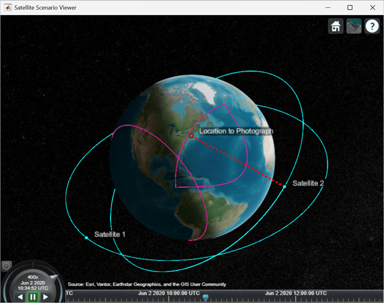
Visualize Scenario
Use satelliteScenarioViewer to launch a satellite scenario viewer and visualize the scenario.
vwr = satelliteScenarioViewer(sc);
Add Access Analysis Between Sensor and Ground Station
Use access to add access analysis between the sensor and location to be photographed. The access analyses determine when each sensor can photograph the site.
ac = access(camSensors,gs);
ac.LineColor = 'magenta';
Visualize Field of View of Sensor
Use fieldOfView to visualize the field of view of each sensor.
fov = fieldOfView(camSensors);
Determine Access Intervals
Use accessIntervals to determine the times when there is access between each sensor and the geographical site. These are the times when the corresponding sensor can photograph the site.
accessIntervals(ac)
ans=3×8 table
              Source                        Target             IntervalNumber         StartTime                EndTime           Duration    StartOrbit    EndOrbit
    ___________________________    ________________________    ______________    ____________________    ____________________    ________    __________    ________

    "Satellite 1 Custom Sensor"    "Location to Photograph"          1           02-Jun-2020 10:48:00    02-Jun-2020 11:16:00      1680          1            2
    "Satellite 2 Custom Sensor"    "Location to Photograph"          1           02-Jun-2020 10:29:00    02-Jun-2020 10:41:00       720          1            1
    "Satellite 2 Custom Sensor"    "Location to Photograph"          2           02-Jun-2020 12:49:00    02-Jun-2020 13:23:00      2040          2            3
Play the satellite scenario with the satellite and ground station.
The scenario achieves visual access for only a portion of the time the ground station is in the field of view of a satellite. This is because of the visibility constraints imposed by the mask elevation angle of the ground station and maximum viewing angles of the conical sensors.
camLat = 30;                           % degrees
camLon = -71;                          % degrees
camHeight = 2e7;                       % meters
campos(vwr,camLat,camLon,camHeight)
play(sc,PlaybackSpeedMultiplier=400)
Algorithms
In order for access to exist:
Between two satellites, line of sight must exist between the two satellites.
Between a satellite and a ground station, line of sight must exist between the two. In addition, the elevation angle of the satellite and the ground station must be greater than the MinElevationAngle of the ground station.
Between two ground stations, line of sight must exist between the two and the elevation angle with respect to one another must be above the MinElevationAngle of the other.
Between a conical sensor not attached to the satellite, line of sight must exist between the conical sensor and the satellite and the satellite must be in the field of view of the conical sensor. The field of view is a region of cone whose vertex is at the conical sensor location and extends indefinitely along the z axis of the cone. The cone angle is defined by the MaxViewAngle of the conical sensor. In addition, if the conical sensor is attached to a ground station (directly or via a gimbal), the elevation angle of the satellite with respect to that ground station must be greater than or equal to each MinElevationAngle of the ground station. There is always access between the conical sensor and the satellite, if the conical sensor is attached to the same satellite
Between two conical sensors not attached to the same satellite, line of sight must exist between the two sensors, and each sensor must be inside the field of view of the other. If a conical sensor is attached to a ground station, the elevation angle of the other conical sensor with respect to the ground station must be greater than or equal to the MinElevationAngle. There is always access between two conical sensors, if the conical sensors are attached to the same satellite or ground station directly or via gimbals
Between a conical sensor not attached to a ground station, there must be line of sight between the two, the elevation angle of the conical sensor with respect to the ground station must be greater than or equal to its MinElevationAngle, and the ground station must be inside the field of view of the sensor. there is always access if the conical sensor is attached to this ground station directly or via a gimbal
Between any two objects, line of sight must not be obstructed by any bodies specified in the
ObstructingBodiesproperty.
Consider these scenarios that illustrate successful and unsuccessful access conditions.
Here, ɑ is the elevation angle of the ground station and β is the maximum view angle (two-sided).
Successful access scenario — Access is successful because:
ɑ is above the
MinElevationAngle,β is less than
MaxViewAngle, andLine-of-sight (LOS) exists between the satellite and the ground station.
Unsuccessful access scenario 1 — Access is unsuccessful even when LOS exists because the satellite is below the minimum view angle of the ground station. In this case, ɑmin <
MinElevationAngle.Unsuccessful access scenario 2 — Access is unsuccessful even when LOS exists because the ground station is outside the field of view of the satellite.
Unsuccessful access scenario 3 — Access is unsuccessful when LOS does not exist. This occurs when the satellite is below the Earth horizon.
The above just described access between two nodes. However, you can have more than two nodes by chaining them, such as going from a ground station to a conical sensor on a satellite, then down to another ground station. In such a case, access must exist between each individual pair of adjacent nodes. For instance:
sc = satelliteScenario;
sat = satellite(sc,10000000,0,0,0,0,0);
c = conicalSensor(sat);
gs1 = groundStation(sc);
gs2 = groundStation(sc,0,0);
ac = access(gs1,c,gs2);
s = accessStatus(ac,sc.StartTime)
s will be true when there is access between gs1 and c, and c and gs2. Also, the following must be true at sc.StartTime:
Line of sight must exist between gs1 and c.
Elevation angle of c with respect to gs1 must be greater than or equal to
MinElevationAngleof gs1.gs1 must be inside the field of view of c.
Line of sight must exist between c and gs2.
Elevation angle of c with respect to gs2 must be greater than or equal to
MinElevationAngleof gs2.gs2 must be inside the field of view of c.
For more information, see Satellite Constellation Access to Ground Station.
Version History
Introduced in R2021a
See Also
Objects
Functions
show|play|hide|groundStation|conicalSensor|transmitter|receiver|satellite