Simulink에서 자전거 로봇의 경로 계획하기
이 예제는 Simulink®에서 주어진 맵의 두 위치 사이에 장애물 없는 경로를 실행하는 방법을 보여줍니다. 경로는 확률적 로드맵(PRM) 계획 알고리즘(mobileRobotPRM))을 사용하여 생성됩니다. 이 경로를 탐색하기 위한 제어 명령은 Pure Pursuit 제어기 블록을 사용하여 만듭니다. 자전거 기구학 모션 모델은 이러한 명령을 기반으로 로봇 모션을 시뮬레이션합니다.
맵 및 Simulink 모델 불러오기
MATLAB 작업 공간에 맵을 불러옵니다
load exampleMaps.mat출발 위치와 목표 위치를 입력합니다
startLoc = [5 5];
goalLoc = [12 3];
가져온 맵은 simpleMap, complexMap, ternaryMap입니다.
Simulink 모델을 엽니다
open_system('pathPlanningBicycleSimulinkModel.slx')모델 개요
모델은 네 가지 주요 작업으로 구성됩니다.
계획
제어
플랜트 모델
계획

Planner MATLAB® Function 블록은 mobileRobotPRM 경로 플래너를 사용하며 시작 위치, 목표 위치, 맵을 입력으로 받습니다. 이 블록은 로봇이 따라가는 웨이포인트로 구성된 배열을 출력합니다. 계획된 웨이포인트는 Pure Pursuit 제어기 블록에서 다운스트림으로 사용됩니다.
제어
Pure Pursuit
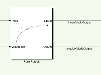
Pure Pursuit 제어기 블록은 웨이포인트와 로봇의 현재 자세를 기반으로 선속도 명령과 각속도 명령을 생성합니다.
목표 도달 여부 검사
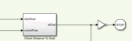
Check Distance to Goal 서브시스템은 목표까지의 현재 거리를 계산하고 임계값 내에 있으면 시뮬레이션을 중지합니다.
플랜트 모델
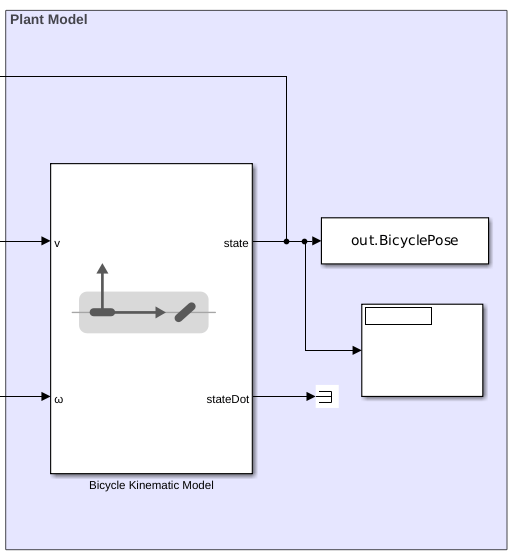
Bicycle Kinematic Model 블록은 단순한 이동체 기구학을 시뮬레이션하는 이동체 모델을 만듭니다. 이 블록은 선속도와 각속도를 Pure Pursuit 제어기 블록의 명령 입력으로 받고 현재 위치 상태와 속도 상태를 출력합니다.
모델 실행하기
모델을 시뮬레이션합니다
simulation = sim('pathPlanningBicycleSimulinkModel.slx');로봇 모션 시각화하기
자세를 확인합니다.
map = binaryOccupancyMap(simpleMap)
map =
  binaryOccupancyMap with properties:

              LayerName: 'binaryLayer'
               DataType: 'logical'
           DefaultValue: 0
             Resolution: 1
               GridSize: [26 27]
    GridLocationInWorld: [0 0]
      GridOriginInLocal: [0 0]
     LocalOriginInWorld: [0 0]
           XLocalLimits: [0 27]
           YLocalLimits: [0 26]
           XWorldLimits: [0 27]
           YWorldLimits: [0 26]
robotPose = simulation.BicyclePose
robotPose = 362×3

    5.0000    5.0000         0
    5.0001    5.0000   -0.0002
    5.0007    5.0000   -0.0012
    5.0036    5.0000   -0.0062
    5.0181    4.9997   -0.0313
    5.0902    4.9929   -0.1569
    5.4081    4.8311   -0.7849
    5.5189    4.6758   -1.1170
    5.5366    4.6356   -1.1930
    5.5512    4.5942   -1.2684
    5.5620    4.5581   -1.2917
    5.5722    4.5217   -1.2971
    5.5868    4.4697   -1.2984
    5.6055    4.4026   -1.2986
    5.6311    4.3108   -1.2985
      ⋮
numRobots = size(robotPose, 2) / 3;
thetaIdx = 3;

% Translation
xyz = robotPose;
xyz(:, thetaIdx) = 0;

% Rotation in XYZ euler angles
theta = robotPose(:,thetaIdx);
thetaEuler = zeros(size(robotPose, 1), 3 * size(theta, 2));
thetaEuler(:, end) = theta;

for k = 1:size(xyz, 1)
    show(map)
    hold on;

    % Plot Start Location
    plotTransforms([startLoc, 0], eul2quat([0, 0, 0]))
    text(startLoc(1), startLoc(2), 2, 'Start');

    % Plot Goal Location
    plotTransforms([goalLoc, 0], eul2quat([0, 0, 0]))
    text(goalLoc(1), goalLoc(2), 2, 'Goal');

    % Plot Robot's XY locations
    plot(robotPose(:, 1), robotPose(:, 2), '-b')

    % Plot Robot's pose as it traverses the path
    quat = eul2quat(thetaEuler(k, :), 'xyz');
    plotTransforms(xyz(k,:), quat, 'MeshFilePath',...
        'groundvehicle.stl');

    pause(0.01)
    hold off;
end
![Figure contains an axes object. The axes object with title Binary Occupancy Grid, xlabel X [meters], ylabel Y [meters] contains 16 objects of type patch, line, image, text.](../../examples/robotics/win64/PlanPathForABicycleRobotInSimulinkExample_05.png)
© Copyright 2019-2020 The MathWorks, Inc.