parabolic

(Not recommended) Solve parabolic PDE problem

parabolic is not recommended. Use solvepde instead.

Syntax

u = parabolic(u0,tlist,model,c,a,f,d)

u = parabolic(u0,tlist,b,p,e,t,c,a,f,d)

u = parabolic(u0,tlist,Kc,Fc,B,ud,M)

u = parabolic(___,rtol)

u = parabolic(___,rtol,atol)

u = parabolic(___,'Stats','off')

Description

Parabolic equation solver

Solves PDE problems of the type

$$d\frac{\partial u}{\partial t}-\nabla \cdot \left(c\nabla u\right)+au=f$$

on a 2-D or 3-D region Ω, or the system PDE problem

$$d\frac{\partial u}{\partial t}-\nabla \cdot \left(c\otimes \nabla u\right)+au=f$$

The variables c, a, f, and d can depend on position, time, and the solution u and its gradient.

u = parabolic(u0,tlist,model,c,a,f,d) produces the solution to the FEM formulation of the scalar PDE problem

$$d\frac{\partial u}{\partial t}-\nabla \cdot \left(c\nabla u\right)+au=f$$

on a 2-D or 3-D region Ω, or the system PDE problem

$$d\frac{\partial u}{\partial t}-\nabla \cdot \left(c\otimes \nabla u\right)+au=f$$

with geometry, mesh, and boundary conditions specified in model, and with initial value u0. The variables c, a, f, and d in the equation correspond to the function coefficients c, a, f, and d respectively.

u = parabolic(u0,tlist,b,p,e,t,c,a,f,d) solves the problem using boundary conditions b and finite element mesh specified in [p,e,t].

u = parabolic(u0,tlist,Kc,Fc,B,ud,M) solves the problem based on finite element matrices that encode the equation, mesh, and boundary conditions.

u = parabolic(___,rtol) and u = parabolic(___,rtol,atol), for any of the previous input arguments, modify the solution process by passing to the ODE solver a relative tolerance rtol, and optionally an absolute tolerance atol.

u = parabolic(___,'Stats','off'), for any of the previous input arguments, turns off the display of internal ODE solver statistics during the solution process.

Examples

Parabolic Equation

Solve the parabolic equation

$$\frac{\partial u}{\partial t}=\Delta u$$

on the square domain specified by squareg.

Create a PDE model and import the geometry.

model = createpde;
geometryFromEdges(model,@squareg);
pdegplot(model,'EdgeLabels','on')
ylim([-1.1,1.1])
axis equal

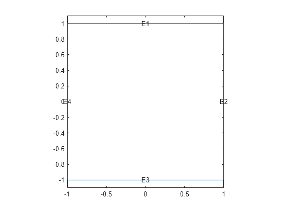
Set Dirichlet boundary conditions $$u=0$$ on all edges.

applyBoundaryCondition(model,'dirichlet',...
                             'Edge',1:model.Geometry.NumEdges, ...
                             'u',0);

Generate a relatively fine mesh.

generateMesh(model,'Hmax',0.02,'GeometricOrder','linear');

Set the initial condition to have $$u(0)=1$$ on the disk $$x^2+y^2\le 0.4^2$$ and $$u(0)=0$$ elsewhere.

p = model.Mesh.Nodes;
u0 = zeros(size(p,2),1); 
ix = find(sqrt(p(1,:).^2 + p(2,:).^2) <= 0.4); 
u0(ix) = ones(size(ix));

Set solution times to be from 0 to 0.1 with step size 0.005.

tlist = linspace(0,0.1,21);

Create the PDE coefficients.

c = 1;
a = 0;
f = 0;
d = 1;

Solve the PDE.

u = parabolic(u0,tlist,model,c,a,f,d);

134 successful steps
0 failed attempts
270 function evaluations
1 partial derivatives
26 LU decompositions
269 solutions of linear systems

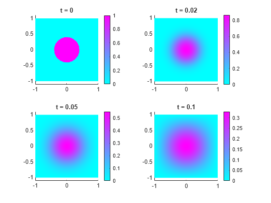
Plot the initial condition, the solution at the final time, and two intermediate solutions.

figure
subplot(2,2,1)
pdeplot(model,'XYData',u(:,1));
axis equal
title('t = 0')
subplot(2,2,2)
pdeplot(model,'XYData',u(:,5))
axis equal
title('t = 0.02')
subplot(2,2,3)
pdeplot(model,'XYData',u(:,11))
axis equal
title('t = 0.05')
subplot(2,2,4)
pdeplot(model,'XYData',u(:,end))
axis equal
title('t = 0.1')

Parabolic Equation Using Legacy Syntax

Solve the parabolic equation

$$\frac{\partial u}{\partial t}=\Delta u$$

on the square domain specified by squareg, using a geometry function to specify the geometry, a boundary function to specify the boundary conditions, and using initmesh to create the finite element mesh.

Specify the geometry as @squareg and plot the geometry.

g = @squareg;
pdegplot(g,'EdgeLabels','on')
ylim([-1.1,1.1])
axis equal

Set Dirichlet boundary conditions $$u=0$$ on all edges. The squareb1 function specifies these boundary conditions.

b = @squareb1;

Generate a relatively fine mesh.

[p,e,t] = initmesh(g,'Hmax',0.02);

Set the initial condition to have $$u(0)=1$$ on the disk $$x^2+y^2\le 0.4^2$$ and $$u(0)=0$$ elsewhere.

u0 = zeros(size(p,2),1); 
ix = find(sqrt(p(1,:).^2 + p(2,:).^2) <= 0.4); 
u0(ix) = ones(size(ix));

Set solution times to be from 0 to 0.1 with step size 0.005.

tlist = linspace(0,0.1,21);

Create the PDE coefficients.

c = 1;
a = 0;
f = 0;
d = 1;

Solve the PDE.

u = parabolic(u0,tlist,b,p,e,t,c,a,f,d);

147 successful steps
0 failed attempts
296 function evaluations
1 partial derivatives
28 LU decompositions
295 solutions of linear systems

Plot the initial condition, the solution at the final time, and two intermediate solutions.

figure
subplot(2,2,1)
pdeplot(p,e,t,'XYData',u(:,1));
axis equal
title('t = 0')
subplot(2,2,2)
pdeplot(p,e,t,'XYData',u(:,5))
axis equal
title('t = 0.02')
subplot(2,2,3)
pdeplot(p,e,t,'XYData',u(:,11))
axis equal
title('t = 0.05')
subplot(2,2,4)
pdeplot(p,e,t,'XYData',u(:,end))
axis equal
title('t = 0.1')

Parabolic Problem Using Matrix Coefficients

Create finite element matrices that encode a parabolic problem, and solve the problem.

The problem is the evolution of temperature in a conducting block. The block is a rectangular slab.

model = createpde(1);
importGeometry(model,'Block.stl');
handl = pdegplot(model,'FaceLabels','on');
view(-42,24)
handl(1).FaceAlpha = 0.5;

Faces 1, 4, and 6 of the slab are kept at 0 degrees. The other faces are insulated. Include the boundary condition on faces 1, 4, and 6. You do not need to include the boundary condition on the other faces because the default condition is insulated.

applyBoundaryCondition(model,'dirichlet','Face',[1,4,6],'u',0);

The initial temperature distribution in the block has the form

$$u_0=10^{-3}xyz.$$

generateMesh(model);
p = model.Mesh.Nodes;
x = p(1,:);
y = p(2,:);
z = p(3,:);
u0 = x.*y.*z*1e-3;

The parabolic equation in toolbox syntax is

$$d\frac{\partial u}{\partial t}-\nabla \cdot (c\nabla u)+au=f.$$

Suppose the thermal conductivity of the block leads to a $$c$$ coefficient value of 1. The values of the other coefficients in this problem are $$d=1$$, $$a=0$$, and $$f=0$$.

d = 1;
c = 1;
a = 0;
f = 0;

Create the finite element matrices that encode the problem.

[Kc,Fc,B,ud] = assempde(model,c,a,f);
[~,M,~] = assema(model,0,d,f);

Solve the problem at time steps of 1 for times ranging from 0 to 40.

tlist = linspace(0,40,41);
u = parabolic(u0,tlist,Kc,Fc,B,ud,M);

35 successful steps
0 failed attempts
72 function evaluations
1 partial derivatives
11 LU decompositions
71 solutions of linear systems

Plot the solution on the outside of the block at times 0, 10, 25, and 40. Ensure that the coloring is the same for all plots.

umin = min(min(u));
umax = max(max(u));
subplot(2,2,1)
pdeplot3D(model,'ColorMapData',u(:,1))
colorbar off
view(125,22)
title 't = 0'
clim([umin umax]);
subplot(2,2,2)
pdeplot3D(model,'ColorMapData',u(:,11))
colorbar off
view(125,22)
title 't = 10'
clim([umin umax]);
subplot(2,2,3)
pdeplot3D(model,'ColorMapData',u(:,26))
colorbar off
view(125,22)
title 't = 25'
clim([umin umax]);
subplot(2,2,4)
pdeplot3D(model,'ColorMapData',u(:,41))
colorbar off
view(125,22)
title 't = 40'
clim([umin umax]);

Input Arguments

u0 — Initial condition

vector | character vector | character array | string scalar | string vector

Initial condition, specified as a scalar, vector of nodal values, character vector, character array, string scalar, or string vector. The initial condition is the value of the solution u at the initial time, specified as a column vector of values at the nodes. The nodes are either p in the [p,e,t] data structure, or are model.Mesh.Nodes.

• If the initial condition is a constant scalar v, specify u0 as v.

• If there are Np nodes in the mesh, and N equations in the system of PDEs, specify u0 as a column vector of Np*N elements, where the first Np elements correspond to the first component of the solution u, the second Np elements correspond to the second component of the solution u, etc.

• Give a text expression of a function, such as 'x.^2 + 5*cos(x.*y)'. If you have a system of N > 1 equations, give a text array such as

  char('x.^2 + 5*cos(x.*y)',...
      'tanh(x.*y)./(1+z.^2)')

Example: x.^2+5*cos(y.*x)

Data Types: double | char | string
Complex Number Support: Yes

tlist — Solution times

real vector

Solution times, specified as a real vector. The solver returns the solution to the PDE at the solution times.

Example: 0:0.2:4

Data Types: double

model — PDE model

PDEModel object

PDE model, specified as a PDEModel object.

Example: model = createpde

c — PDE coefficient

scalar | matrix | character vector | character array | string scalar | string vector | coefficient function

PDE coefficient, specified as a scalar, matrix, character vector, character array, string scalar, string vector, or coefficient function. c represents the c coefficient in the scalar PDE

$$d\frac{\partial u}{\partial t}-\nabla \cdot \left(c\nabla u\right)+au=f$$

or in the system of PDEs

$$d\frac{\partial u}{\partial t}-\nabla \cdot \left(c\otimes \nabla u\right)+au=f$$

Example: 'cosh(x+y.^2)'

Data Types: double | char | string | function_handle
Complex Number Support: Yes

a — PDE coefficient

scalar | matrix | character vector | character array | string scalar | string vector | coefficient function

PDE coefficient, specified as a scalar, matrix, character vector, character array, string scalar, string vector, or coefficient function. a represents the a coefficient in the scalar PDE

$$d\frac{\partial u}{\partial t}-\nabla \cdot \left(c\nabla u\right)+au=f$$

or in the system of PDEs

$$d\frac{\partial u}{\partial t}-\nabla \cdot \left(c\otimes \nabla u\right)+au=f$$

Example: 2*eye(3)

Data Types: double | char | string | function_handle
Complex Number Support: Yes

f — PDE coefficient

scalar | matrix | character vector | character array | string scalar | string vector | coefficient function

PDE coefficient, specified as a scalar, matrix, character vector, character array, string scalar, string vector, or coefficient function. f represents the f coefficient in the scalar PDE

$$d\frac{\partial u}{\partial t}-\nabla \cdot \left(c\nabla u\right)+au=f$$

or in the system of PDEs

$$d\frac{\partial u}{\partial t}-\nabla \cdot \left(c\otimes \nabla u\right)+au=f$$

Example: char('sin(x)';'cos(y)';'tan(z)')

Data Types: double | char | string | function_handle
Complex Number Support: Yes

d — PDE coefficient

scalar | matrix | character vector | character array | string scalar | string vector | coefficient function

PDE coefficient, specified as a scalar, matrix, character vector, character array, string scalar, string vector, or coefficient function. d represents the d coefficient in the scalar PDE

$$d\frac{\partial u}{\partial t}-\nabla \cdot \left(c\nabla u\right)+au=f$$

or in the system of PDEs

$$d\frac{\partial u}{\partial t}-\nabla \cdot \left(c\otimes \nabla u\right)+au=f$$

Example: 2*eye(3)

Data Types: double | char | string | function_handle
Complex Number Support: Yes

b — Boundary conditions

boundary matrix | boundary file

Boundary conditions, specified as a boundary matrix or boundary file. Pass a boundary file as a function handle or as a file name. A boundary matrix is generally an export from the PDE Modeler app.

Example: b = 'circleb1', b = "circleb1", or b = @circleb1

Data Types: double | char | string | function_handle

p — Mesh points

matrix

Mesh points, specified as a 2-by-Np matrix of points, where Np is the number of points in the mesh. For a description of the (p,e,t) matrices, see Mesh Data as [p,e,t] Triples.

Typically, you use the p, e, and t data exported from the PDE Modeler app, or generated by initmesh or refinemesh.

Example: [p,e,t] = initmesh(gd)

Data Types: double

e — Mesh edges

matrix

Mesh edges, specified as a 7-by-Ne matrix of edges, where Ne is the number of edges in the mesh. For a description of the (p,e,t) matrices, see Mesh Data as [p,e,t] Triples.

Typically, you use the p, e, and t data exported from the PDE Modeler app, or generated by initmesh or refinemesh.

Example: [p,e,t] = initmesh(gd)

Data Types: double

t — Mesh triangles

matrix

Mesh triangles, specified as a 4-by-Nt matrix of triangles, where Nt is the number of triangles in the mesh. For a description of the (p,e,t) matrices, see Mesh Data as [p,e,t] Triples.

Typically, you use the p, e, and t data exported from the PDE Modeler app, or generated by initmesh or refinemesh.

Example: [p,e,t] = initmesh(gd)

Data Types: double

Kc — Stiffness matrix

sparse matrix | full matrix

Stiffness matrix, specified as a sparse matrix or as a full matrix. See Elliptic Equations. Typically, Kc is the output of assempde.

Fc — Load vector

vector

Load vector, specified as a vector. See Elliptic Equations. Typically, Fc is the output of assempde.

B — Dirichlet nullspace

sparse matrix

Dirichlet nullspace, returned as a sparse matrix. See Algorithms. Typically, B is the output of assempde.

ud — Dirichlet vector

vector

Dirichlet vector, returned as a vector. See Algorithms. Typically, ud is the output of assempde.

M — Mass matrix

sparse matrix | full matrix

Mass matrix. specified as a sparse matrix or a full matrix. See Elliptic Equations.

To obtain the input matrices for pdeeig, hyperbolic or parabolic, run both assema and assempde:

[Kc,Fc,B,ud] = assempde(model,c,a,f);
[~,M,~] = assema(model,0,d,f);

Note

Create the M matrix using assema with d, not a, as the argument before f.

Data Types: double
Complex Number Support: Yes

rtol — Relative tolerance for ODE solver

1e-3 (default) | positive real

Relative tolerance for ODE solver, specified as a positive real.

Example: 2e-4

Data Types: double

atol — Absolute tolerance for ODE solver

1e-6 (default) | positive real

Absolute tolerance for ODE solver, specified as a positive real.

Example: 2e-7

Data Types: double

Output Arguments

u — PDE solution

matrix

PDE solution, returned as a matrix. The matrix is Np*N-by-T, where Np is the number of nodes in the mesh, N is the number of equations in the PDE (N = 1 for a scalar PDE), and T is the number of solution times, meaning the length of tlist. The solution matrix has the following structure.

• The first Np elements of each column in u represent the solution of equation 1, then next Np elements represent the solution of equation 2, etc. The solution u is the value at the corresponding node in the mesh.

• Column i of u represents the solution at time tlist(i).

To obtain the solution at an arbitrary point in the geometry, use pdeInterpolant.

Algorithms

Reducing Parabolic Equations to Elliptic Equations

parabolic internally calls assema, assemb, and assempde to create finite element matrices corresponding to the problem. It calls ode15s to solve the resulting system of ordinary differential equations.

Partial Differential Equation Toolbox™ solves equations of the form

$$m\frac{{\partial }^{2}u}{\partial t^2}+d\frac{\partial u}{\partial t}-\nabla ·\left(c\nabla u\right)+au=f$$

When the m coefficient is 0, but d is not, the documentation refers to the equation as parabolic, whether or not it is mathematically in parabolic form.

A parabolic problem is to solve the equation

$$d\frac{\partial u}{\partial t}-\nabla \cdot \left(c\nabla u\right)+au=f\text{in }\Omega$$

with the initial condition

u(x,0) = u₀(x) for x∊Ω

where x represents a 2-D or 3-D point and there are boundary conditions of the same kind as for the elliptic equation on ∂Ω.

The heat equation reads

$$\rho C\frac{\partial u}{\partial t}-\nabla ·\left(k\nabla u\right)+h\left(u-u_{\infty }\right)=f$$

in the presence of distributed heat loss to the surroundings. ρ is the density, C is the thermal capacity, k is the thermal conductivity, h is the film coefficient, u_∞ is the ambient temperature, and f is the heat source.

For time-independent coefficients, the steady-state solution of the equation is the solution to the standard elliptic equation

–∇ · (c∇u) + au = f.

Assuming a mesh on Ω and t ≥ 0, expand the solution to the PDE (as a function of x) in the Finite Element Method basis:

$$u(x,t)={\displaystyle \sum _i{U}_i(t){\varphi }_i(x)}$$

Plugging the expansion into the PDE, multiplying with a test function ϕ_j, integrating over Ω, and applying Green's formula and the boundary conditions yield

$$\begin{array}{l}{\displaystyle \sum _i{\displaystyle \underset{\Omega }{\int }d{\varphi }_j{\varphi }_i\frac{d{U}_i\left(t\right)}{dt}}}dx+{\displaystyle \sum _i\left({\displaystyle \underset{\Omega }{\int }\left(\nabla {\varphi }_j\cdot \left(c\nabla {\varphi }_i\right)+a{\varphi }_j{\varphi }_i\right)dx+{\displaystyle \underset{\partial \Omega }{\int }q{\varphi }_j{\varphi }_{i}ds}}\right)U_i(t)}\\ ={\displaystyle \underset{\Omega }{\int }f{\varphi }_{j}dx}+{\displaystyle \underset{\partial \Omega }{\int }g{\varphi }_{j}ds}\forall j\end{array}$$

In matrix notation, we have to solve the linear, large and sparse ODE system

$$M\frac{dU}{dt}+KU=F$$

This method is traditionally called method of lines semidiscretization.

Solving the ODE with the initial value

U_i(0) = u₀(x_i)

yields the solution to the PDE at each node x_i and time t. Note that K and F are the stiffness matrix and the right-hand side of the elliptic problem

–∇ · (c∇u) + au = f in Ω

with the original boundary conditions, while M is just the mass matrix of the problem

–∇ · (0∇u) + du = 0 in Ω.

When the Dirichlet conditions are time dependent, F contains contributions from time derivatives of h and r. These derivatives are evaluated by finite differences of the user-specified data.

The ODE system is ill conditioned. Explicit time integrators are forced by stability requirements to very short time steps while implicit solvers can be expensive since they solve an elliptic problem at every time step. The numerical integration of the ODE system is performed by the MATLAB^® ODE Suite functions, which are efficient for this class of problems. The time step is controlled to satisfy a tolerance on the error, and factorizations of coefficient matrices are performed only when necessary. When coefficients are time dependent, the necessity of reevaluating and refactorizing the matrices each time step may still make the solution time consuming, although parabolic reevaluates only that which varies with time. In certain cases a time-dependent Dirichlet matrix h(t) may cause the error control to fail, even if the problem is mathematically sound and the solution u(t) is smooth. This can happen because the ODE integrator looks only at the reduced solution v with u = Bv + ud. As h changes, the pivoting scheme employed for numerical stability may change the elimination order from one step to the next. This means that B, v, and ud all change discontinuously, although u itself does not.

Version History

Introduced before R2006a

R2016a: Not recommended

parabolic is not recommended. Use solvepde instead. There are no plans to remove parabolic.

R2012b: Coefficients of parabolic PDEs as functions of the solution and its gradient

You can now solve parabolic equations whose coefficients depend on the solution u or on the gradient of u.