Follow Equation Solution as a Parameter Changes
This example shows how to solve an equation repeatedly as a parameter changes by starting subsequent solutions from the previous solution point. Often, this process leads to efficient solutions. However, a solution can sometimes disappear, requiring a start from a new point or points.
Parameterized Scalar Equation
The parameterized equation to solve is
,
where is a numeric parameter that goes from 0 to 5. At , one solution to this equation is . When is not too large in absolute value, the equation has three solutions. To visualize the equation, create the left side of the equation as an anonymous function. Plot the function.
fun = @(x)sinh(x) - 3*x;
t = linspace(-3.5,3.5);
plot(t,fun(t),t,zeros(size(t)),"k-")
xlabel("x")
ylabel("fun(x)")
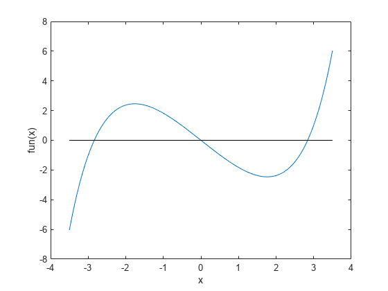
When is too large or too small, there is only one solution.
Problem-Based Setup
To create an objective function for the problem-based approach, create an optimization expression expr in an optimization variable x.
x = optimvar("x");
expr = sinh(x) - 3*x;
Create and Plot Solutions
Starting from the initial solution at , find solutions for 100 values of from 0 through 5. Because fun is a scalar nonlinear function, solve calls fzero as the solver.
Set up the problem object, options, and data structures for holding solution statistics.
prob = eqnproblem;
options = optimset(Display="off");
sols = zeros(100,1);
fevals = sols;
as = linspace(0,5);
Solve the equation in a loop, starting from the first solution sols(1) = 0.
for i = 2:length(as)
    x0.x = sols(i-1); % Start from previous solution
    prob.Equations = expr == as(i);
    [sol,~,~,output] = solve(prob,x0,Options=options);
    sols(i) = sol.x;
    fevals(i) = output.funcCount;
end
Plot the solution as a function of the parameter a and the number of function evaluations taken to reach the solution.
subplot(2,1,1)
plot(as,sols,"ko")
xlabel("a")
ylabel("Solution(x)")
subplot(2,1,2)
plot(fevals,"k*")
xlabel("Iteration Number")
ylabel("Fevals")
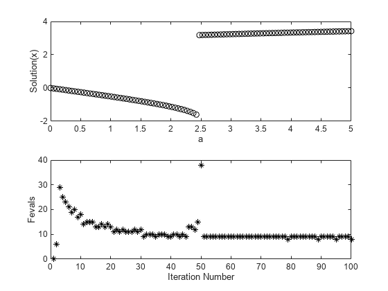
A jump in the solution occurs near . At the same point, the number of function evaluations to reach a solution increases from near 15 to near 40. To understand why, examine a more detailed plot of the function. Plot the function and every seventh solution point.
figure
t = linspace(-3.5,3.5);
plot(t,fun(t));
hold on
plot([-3.5,min(sols)],[2.5,2.5],"k--")
legend("fun","Maximum a",Location="north",autoupdate="off")
for a0 = 7:7:100
    plot(sols(a0),as(a0),"ro")
    if mod(a0,2) == 1
        text(sols(a0) + 0.15,as(a0) + 0.15,num2str(a0/7))
    else
        text(sols(a0) - 0.3,as(a0) + 0.05,num2str(a0/7))
    end
end
plot(t,zeros(size(t)),"k-")
hold off
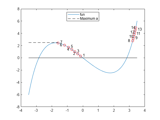
As increases, at first the solutions move to the left. However, when is above 2.5, there is no longer a solution near the previous solution. fzero requires extra function evaluations to search for a solution, and finds a solution near x = 3. After that, the solution values move slowly to the right as increases further. The solver requires only about 10 function evaluations for each subsequent solution.
Choose Different Solver
The fsolve solver can be more efficient than fzero. However, fsolve can become stuck in a local minimum and fail to solve the equation.
Set up the problem object, options, and data structures for holding solution statistics.
probfsolve = eqnproblem;
sols = zeros(100,1);
fevals = sols;
infeas = sols;
asfsolve = linspace(0,5);
Solve the equation in a loop, starting from the first solution sols(1) = 0.
for i = 2:length(as)
    x0.x = sols(i-1); % Start from previous solution
    probfsolve.Equations = expr == asfsolve(i);
    [sol,fval,~,output] = solve(probfsolve,x0,Options=options,Solver="fsolve");
    sols(i) = sol.x;
    fevals(i) = output.funcCount;
    infeas(i) = fval;
end
Plot the solution as a function of the parameter a and the number of function evaluations taken to reach the solution.
figure
subplot(2,1,1)
plot(asfsolve,sols,"ko",asfsolve,infeas,"r-")
xlabel("a")
legend("Solution","Error of Solution",Location="best")
subplot(2,1,2)
plot(fevals,"k*")
xlabel("Iteration Number")
ylabel("Fevals")
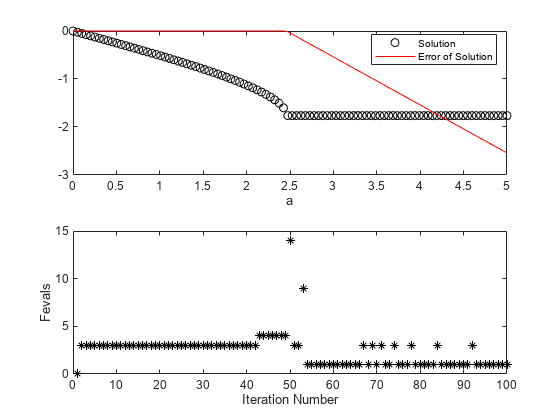
fsolve is somewhat more efficient than fzero, requiring about 7 or 8 function evaluations per iteration. Again, when the solver finds no solution near the previous value, the solver requires many more function evaluations to search for a solution. This time, the search is unsuccessful. Subsequent iterations require few function evaluations for the most part, but fail to find a solution. The Error of Solution plot shows the function value .
To try to overcome a local minimum not being a solution, search again from a different start point when fsolve returns with a negative exit flag. Set up the problem object, options, and data structures for holding solution statistics.
rng default % For reproducibility
sols = zeros(100,1);
fevals = sols;
asfsolve = linspace(0,5);
Solve the equation in a loop, starting from the first solution sols(1) = 0.
for i = 2:length(as)
    x0.x = sols(i-1); % Start from previous solution
    probfsolve.Equations = expr == asfsolve(i);
    [sol,~,exitflag,output] = solve(probfsolve,x0,Options=options,Solver="fsolve");

    while exitflag <= 0 % If fsolve fails to find a solution
        x0.x = 5*randn; % Try again from a new start point
        fevals(i) = fevals(i) + output.funcCount;
        [sol,~,exitflag,output] = solve(probfsolve,x0,Options=options,Solver="fsolve");
    end

    sols(i) = sol.x;
    fevals(i) = fevals(i) + output.funcCount;
end
Plot the solution as a function of the parameter a and the number of function evaluations taken to reach the solution.
figure
subplot(2,1,1)
plot(asfsolve,sols,"ko")
xlabel("a")
ylabel("Solution(x)")
subplot(2,1,2)
plot(fevals,"k*")
xlabel("Iteration Number")
ylabel("Fevals")

This time, fsolve recovers from the poor initial point near and obtains a solution similar to the one obtained by fzero. The number of function evaluations for each iteration is typically 8, increasing to about 15 at the point where the solution jumps.
Convert Objective Function Using fcn2optimexpr
For some objective functions or software versions, you must convert nonlinear functions to optimization expressions by using fcn2optimexpr. See Supported Operations for Optimization Variables and Expressions and Convert Nonlinear Function to Optimization Expression. For this example, convert the original function fun used for plotting to the optimization expression expr:
expr = fcn2optimexpr(fun,x);
The remainder of the example is exactly the same after this change to the definition of expr.