GNSS 시뮬레이션 개요

GNSS(범지구 위성 항법 시스템) 시뮬레이션은 수신기 위치 추정값을 생성합니다. 이러한 수신기 위치 추정값은 GPS 센서 모델과 GNSS 센서 모델에서 gpsSensor 객체와 gnssSensor 객체로 가져옵니다. DOP(dilution of precision) 출력값을 사용하여 gnssSensor의 위치 추정값 상태를 모니터링하고 사용 가능한 위성 개수를 비교합니다.

시뮬레이션 파라미터

GNSS 시뮬레이션에 사용할 파라미터를 지정합니다.

• GNSS 수신기의 샘플링 레이트

• 로컬 내비게이션 기준 프레임

• LLA(위도, 경도, 고도) 좌표계에서의 지구상 위치

• 시뮬레이션할 샘플 개수

Fs = 1;
refFrame = "NED";
lla0 = [42.2825 -71.343 53.0352];
N = 100;

정지 상태인 센서에 대한 궤적을 만듭니다.

pos = zeros(N, 3);
vel = zeros(N, 3);
time = (0:N-1) ./ Fs;

센서 모델 생성

각각에 대해 동일한 초기 파라미터를 사용하여 GNSS 시뮬레이션 객체인 gpsSensor 및 gnssSensor를 생성합니다.

gps = gpsSensor("SampleRate", Fs, "ReferenceLocation", lla0, ...
    "ReferenceFrame", refFrame);

gnss = gnssSensor("SampleRate", Fs, "ReferenceLocation", lla0, ...
    "ReferenceFrame", refFrame);

gpsSensor를 사용한 시뮬레이션

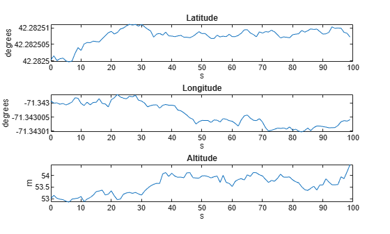
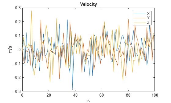
GPS 센서를 사용하여 정지 상태인 수신기에서 출력값을 생성합니다. LLA 좌표계에서의 위치와 각 방향에서의 속도를 시각화합니다.

% Generate outputs.
[llaGPS, velGPS] = gps(pos, vel);

% Visualize position.
figure
subplot(3, 1, 1)
plot(time, llaGPS(:,1))
title('Latitude')
ylabel('degrees')
xlabel('s')
subplot(3, 1, 2)
plot(time, llaGPS(:,2))
title('Longitude')
ylabel('degrees')
xlabel('s')
subplot(3, 1, 3)
plot(time, llaGPS(:,3))
title('Altitude')
ylabel('m')
xlabel('s')

% Visualize velocity.
figure
plot(time, velGPS)
title('Velocity')
legend('X', 'Y', 'Z')
ylabel('m/s')
xlabel('s')

gnssSensor를 사용한 시뮬레이션

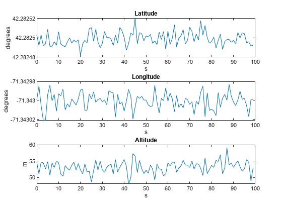
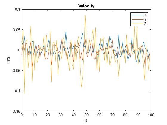
GNSS 센서를 사용하여 정지 상태인 수신기에서 출력값을 생성합니다. 위치와 속도를 시각화하여 시뮬레이션에서 차이가 있음을 확인합니다.

% Generate outputs.
[llaGNSS, velGNSS] = gnss(pos, vel);

% Visualize positon.
figure
subplot(3, 1, 1)
plot(time, llaGNSS(:,1))
title('Latitude')
ylabel('degrees')
xlabel('s')
subplot(3, 1, 2)
plot(time, llaGNSS(:,2))
title('Longitude')
ylabel('degrees')
xlabel('s')
subplot(3, 1, 3)
plot(time, llaGNSS(:,3))
title('Altitude')
ylabel('m')
xlabel('s')

% Visualize velocity.
figure
plot(time, velGNSS)
title('Velocity')
legend('X', 'Y', 'Z')
ylabel('m/s')
xlabel('s')

DOP(Dilution of Precision)

gnssSensor 객체는 gpsSensor 객체에 비해 시뮬레이션 충실도가 더 높습니다. 예를 들어 gnssSensor 객체는 시뮬레이션된 위성 위치를 사용하여 수신기 위치를 추정합니다. 이는 위치 추정값과 더불어 HDOP(horizontal dilution of precision)와 VDOP(vertical dilution of precision)를 보고할 수 있다는 의미입니다. 이 값들은 위성의 기하 배치를 바탕으로 위치 추정값이 얼마나 정확한지 나타냅니다. 값이 작을수록 더 정확한 추정값을 의미합니다.

% Set the RNG seed to reproduce results. 
rng('default')

% Specify the start time of the simulation.
initTime = datetime(2020, 4, 20, 18, 10, 0, "TimeZone", "America/New_York");

% Create the GNSS receiver model.
gnss = gnssSensor("SampleRate", Fs, "ReferenceLocation", lla0, ...
    "ReferenceFrame", refFrame, "InitialTime", initTime);

% Obtain the receiver status. 
[~, ~, status] = gnss(pos, vel);
disp(status(1))

      SatelliteAzimuth: [7x1 double]
    SatelliteElevation: [7x1 double]
                  HDOP: 1.1290
                  VDOP: 1.9035

시뮬레이션 전체 과정의 HDOP를 표시합니다. HDOP에 감소가 있습니다. 이는 위성 기하가 변경되었음을 의미합니다.

hdops = vertcat(status.HDOP);

figure
plot(time, vertcat(status.HDOP))
title('HDOP')
ylabel('m')
xlabel('s')

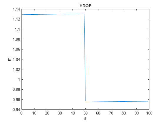
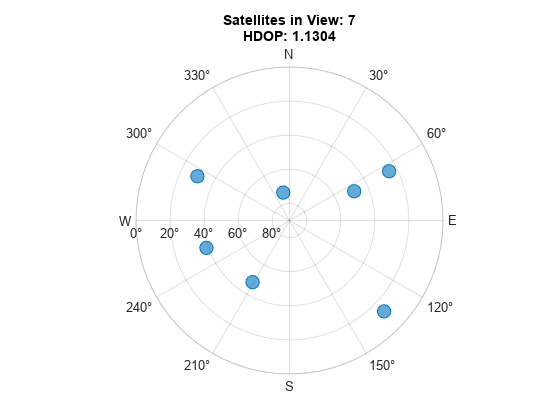
위성 기하가 변경되었는지 확인합니다. HDOP가 감소된 인덱스를 찾아서 이것이 표시되는 위성 개수의 변화와 상응하는지 확인합니다. numSats 변수가 7에서 8로 늘어납니다.

% Find expected sample index for a change in the
% number of satellites in view.
[~, satChangeIdx] = max(abs(diff(hdops)));

% Visualize the satellite geometry before the
% change in HDOP.
satAz = status(satChangeIdx).SatelliteAzimuth;
satEl = status(satChangeIdx).SatelliteElevation;
numSats = numel(satAz);
skyplot(satAz, satEl);
title(sprintf('Satellites in View: %d\nHDOP: %.4f', ...
    numSats, hdops(satChangeIdx)))

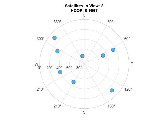
% Visualize the satellite geometry after the
% change in HDOP.
satAz = status(satChangeIdx+1).SatelliteAzimuth;
satEl = status(satChangeIdx+1).SatelliteElevation;
numSats = numel(satAz);
skyplot(satAz, satEl);
title(sprintf('Satellites in View: %d\nHDOP: %.4f', ...
    numSats, hdops(satChangeIdx+1)))

GNSS 수신기 위치 추정값에 칼만 필터를 사용하는 다른 센서 측정값을 결합할 때 HDOP 값과 VDOP 값을 측정 공분산 행렬의 대각선 요소로 사용할 수 있습니다.

% Convert HDOP and VDOP to a measurement covariance matrix.
hdop = status(1).HDOP;
vdop = status(1).VDOP;
measCov = diag([hdop.^2/2, hdop.^2/2, vdop.^2]);
disp(measCov)

    0.6373         0         0
         0    0.6373         0
         0         0    3.6233