Model Predictive Control of a Multi-Input Multi-Output Nonlinear Plant
This example shows how to design a model predictive controller for a multi-input multi-output nonlinear plant defined in Simulink® and simulate the closed loop. The plant has three manipulated variables and two measured outputs.
Linearize the Nonlinear Plant
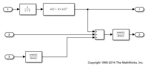
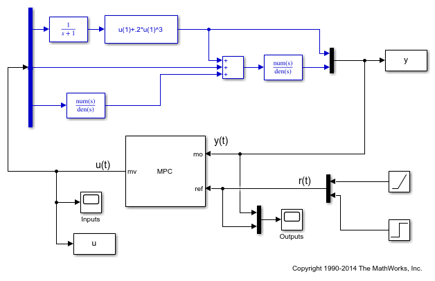
The nonlinear plant is implemented in the Simulink model mpc_nonlinmodel. Notice the nonlinearity 0.2*u(1)^3 from the first input to the first output.
open('mpc_nonlinmodel')
ans =

  logical

   1
Linearize the plant at the default operating conditions (the initial states of the transfer function blocks are all zero) using the linearize command from Simulink® Control Design™.
plant = linearize('mpc_nonlinmodel');
Assign names to I/O variables.
plant.InputName = {'Mass Flow';'Heat Flow';'Pressure'};
plant.OutputName = {'Temperature';'Level'};
plant.InputUnit = {'kg/s' 'J/s' 'Pa'};
plant.OutputUnit = {'K' 'm'};
Note that since you have not defined any measured or unmeasured disturbance, or any an unmeasured output, when an MPC controller is created based on plant, by default all plant inputs are assumed to be manipulated variables and all plant outputs are assumed to be measured outputs.
Design the MPC Controller
Create the controller object with sampling period, prediction and control horizons of 0.2 sec, 5 steps, and 2 moves, respectively;
mpcobj = mpc(plant,0.2,5,2);
-->"Weights.ManipulatedVariables" is empty. Assuming default 0.00000.
-->"Weights.ManipulatedVariablesRate" is empty. Assuming default 0.10000.
-->"Weights.OutputVariables" is empty. Assuming default 1.00000.
Specify hard constraints on the manipulated variable.
mpcobj.MV = struct('Min',{-3;-2;-2},'Max',{3;2;2},'RateMin',{-1000;-1000;-1000});
Define weights on manipulated variables and output signals.
mpcobj.Weights = struct('MV',[0 0 0],'MVRate',[.1 .1 .1],'OV',[1 1]);
Display the MPC object to review its properties.
mpcobj
MPC object (created on 19-Apr-2026 09:57:57):
---------------------------------------------
Sampling time:      0.2 (seconds)
Prediction Horizon: 5
Control Horizon:    2

Plant Model:
                                      --------------
      3  manipulated variable(s)   -->|  5 states  |
                                      |            |-->  2 measured output(s)
      0  measured disturbance(s)   -->|  3 inputs  |
                                      |            |-->  0 unmeasured output(s)
      0  unmeasured disturbance(s) -->|  2 outputs |
                                      --------------
Disturbance and Noise Models:
        Output disturbance model: default (type "getoutdist(mpcobj)" for details)
         Measurement noise model: default (unity gain after scaling)

Weights:
        ManipulatedVariables: [0 0 0]
    ManipulatedVariablesRate: [0.1000 0.1000 0.1000]
             OutputVariables: [1 1]
                         ECR: 100000

State Estimation:  Default Kalman Filter (type "getEstimator(mpcobj)" for details)

Constraints:
 -3 <= Mass Flow (kg/s) <= 3, -1000 <= Mass Flow/rate (kg/s) <= Inf, Temperature (K) is unconstrained
  -2 <= Heat Flow (J/s) <= 2,  -1000 <= Heat Flow/rate (J/s) <= Inf,       Level (m) is unconstrained
    -2 <= Pressure (Pa) <= 2,    -1000 <= Pressure/rate (Pa) <= Inf

Use built-in "active-set" QP solver with MaxIterations of 120.
Simulate the Closed Loop Using Simulink
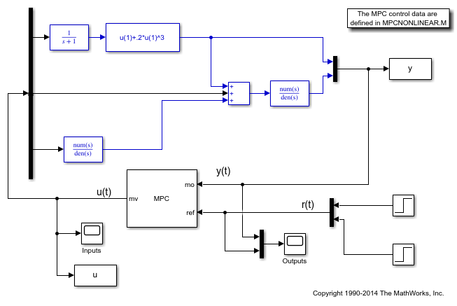
Open the pre-existing Simulink model for the closed-loop simulation. The plant model is identical to the one used for linearization, while the MPC controller is implemented with an MPC controller block, which has the workspace MPC object mpcobj as parameter. The reference for the first output is a step signal rising from zero to one for t=0, as soon as the simulation starts. The reference for the second output
mdl1 = 'mpc_nonlinear';
open_system(mdl1)
Run the closed loop simulation.
sim(mdl1)
-->Converting model to discrete time.
-->Integrator added as output disturbance model for measured output #1.
-->Integrator added as output disturbance model for measured output #2.
-->"Model.Noise" is empty. Assuming white noise on each measured output.
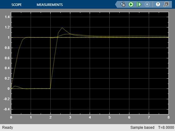
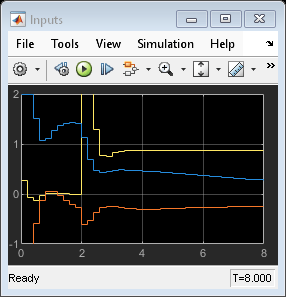
Despite the presence of the nonlinearity, both outputs track their references well after a few seconds, while, as expected, the manipulated variables stay within the preset hard constraints.
Modify MPC Design to Track Ramp Signals
In order to both track a ramp while compensating for the nonlinearity, define a disturbance model on both outputs as a triple integrator (without the nonlinearity a double integrator would suffice).
outdistmodel = tf({1 0;0 1},{[1 0 0 0],1;1,[1 0 0 0]});
setoutdist(mpcobj,'model',outdistmodel);
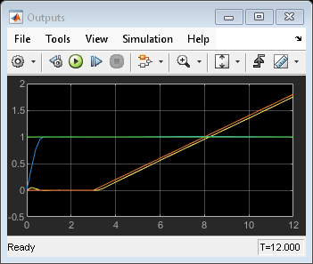
Open the pre-existing Simulink model for the closed-loop simulation. It is identical to the previous closed loop model, except for the fact that the reference for the first plant output is no longer a step but a ramp signal that rises with slope of 0.2 after 3 seconds.
mdl2 = 'mpc_nonlinear_setoutdist';
open_system(mdl2)
Run the closed loop simulation for 12 seconds.
sim(mdl2,12)
-->Converting model to discrete time.
-->"Model.Noise" is empty. Assuming white noise on each measured output.

Simulate Without Constraints
When the constraints are not active, the MPC controller behaves like a linear controller. Simulate two versions of an unconstrained MPC controller in closed loop to illustrate this fact.
First, remove the constraints from mcpobj.
mpcobj.MV = [];
Then reset the output disturbance model to default, (this is only done to get a simpler version of a linear MPC controller in the next step).
setoutdist(mpcobj,'integrators');
Convert the unconstrained MPC controller to a linear time invariant (LTI) state space dynamic system, having the vector [ym;r] as input, where ym is the vector of measured output signals (at a given step), and r is the vector of output references (at the same given step).
LTI = ss(mpcobj,'r'); % use reference as additional input signal
-->Converting model to discrete time.
-->Integrator added as output disturbance model for measured output #1.
-->Integrator added as output disturbance model for measured output #2.
-->"Model.Noise" is empty. Assuming white noise on each measured output.
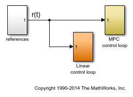
Open the pre-existing Simulink model for the closed-loop simulation. The "references" block contains two step signals (acting after 4 and 0 seconds, respectively) that are used as a reference. The "MPC control loop" block is equivalent to the first closed loop, except for the fact that the reference signals are supplied to it as input. The "Linear control loop" block is equivalent to the "MPC control loop" block except for the fact that the controller is an LTI block having the workspace ss object LTI as parameter.
refs = [1;1];                  % set values for step signal references
mdl3 = 'mpc_nonlinear_ss';
open_system(mdl3)
Run the closed loop simulation for 12 seconds.
sim(mdl3)
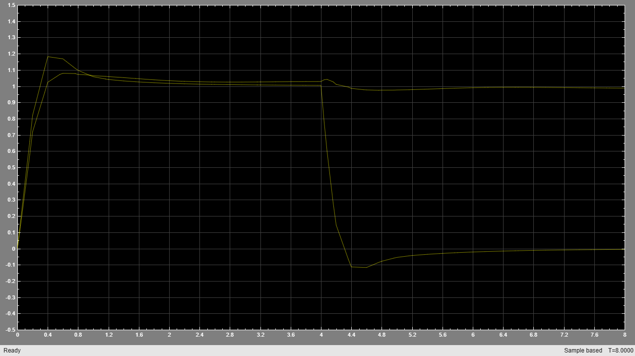
The inputs and outputs signals look identical for both loops. Also note that the manipulated variable are no longer bounded by the previous constraints.
Compare Simulation Results
fprintf('Compare output trajectories: ||ympc-ylin|| = %g\n',norm(ympc-ylin));
% The MPC controller and the linear controller produce the same closed-loop
% trajectories.
Compare output trajectories: ||ympc-ylin|| = 1.4807e-14
As expected, there is only a negligible difference due to numerical errors.
See Also
Apps
Functions
linearize(Simulink Control Design)