Detect Lines Using Radon Transform
This example shows how to use the Radon transform to detect lines in an image. The Radon transform is closely related to a common computer vision operation known as the Hough transform. You can use the radon function to implement a form of the Hough transform used to detect straight lines.
Compute the Radon Transform of an Image
Read an image into the workspace. Convert it into a grayscale image.
I = fitsread("solarspectra.fts");
I = rescale(I);
Display the original image.
figure
imshow(I)
title("Original Image")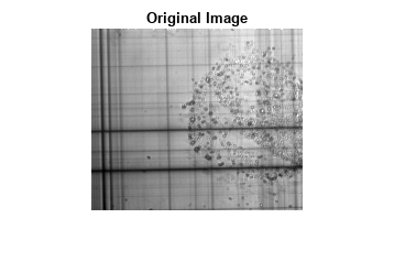
Compute a binary edge image using the edge function. Display the binary image returned by the edge function.
BW = edge(I);
figure
imshow(BW)
title("Edges of Original Image")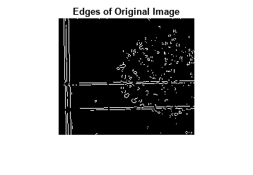
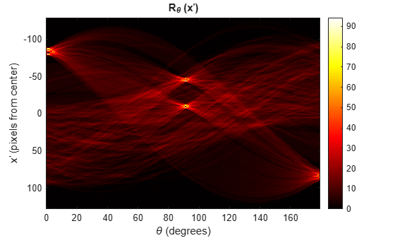
Calculate the Radon transform of the image, using the radon function. The locations of peaks in the transform correspond to the locations of straight lines in the original image.
theta = 0:179;
[R,xp] = radon(BW,theta);
Display the result of the Radon transform.
figure
imagesc(theta,xp,R)
colormap(hot)
xlabel("\theta (degrees)")
ylabel("x^{\prime} (pixels from center)")
title("R_{\theta} (x^{\prime})")
colorbar
Interpret the Peaks of the Radon Transform
Calculate the θ and x' offset values for the five largest peaks. The xp_peak_offset values represent the offset of the peak from the center of the image, in pixels.
R_sort = sort(unique(R),"descend");
[row_peak,col_peak] = find(ismember(R,R_sort(1:5)));
xp_peak_offset = xp(row_peak);
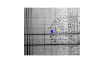
theta_peak = theta(col_peak);Add an x marker at the center of the original image. The row indices of an image map to the y-direction, and the columns map to the x-direction, so calculate centerX as half the number of columns and centerY as half the number of rows in the image I.
centerX = ceil(size(I,2)/2);
centerY = ceil(size(I,1)/2);

figure
imshow(I)
hold on
scatter(centerX,centerY,50,"bx",LineWidth=2)
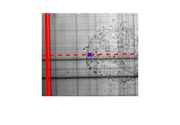
There are three strong peaks with θ = 1 degree and offsets of –80, –84, and –87 pixels from center. Plot the radial line that passes through the center at an angle of θ = 1 degree as a red dashed line. Represent the Radon as solid red lines that are perpendicular to the dashed line, and shifted –80, –84, and –87 pixels from the center, which positions them to the left.
[x1,y1] = pol2cart(deg2rad(1),5000);
plot([centerX-x1 centerX+x1],[centerY+y1 centerY-y1],"r--",LineWidth=2)

[x91,y91] = pol2cart(deg2rad(91),100);
for i=1:3
    plot([centerX-x91+xp_peak_offset(i) centerX+x91+xp_peak_offset(i)], ...
        [centerY+y91 centerY-y91], ...
        "r",LineWidth=2)
end
There are also two strong peaks at θ = 91 degrees, with offsets of –8 and –44 pixels from center. Plot the radial line that passes through the center at an angle of θ = 91 degrees as a green dashed line. Represent the Radon peaks as solid green lines that are perpendicular to the dashed line, and shifted –8 and –44 pixels from center, which positions them down.
plot([centerX-x91 centerX+x91],[centerY+y91 centerY-y91],"g--",LineWidth=2)

for i=4:5
plot([centerX-x1 centerX+x1], ...
    [centerY+y1-xp_peak_offset(i) centerY-y1-xp_peak_offset(i)], ...
    "g",LineWidth=2)
end
