Portfolio Optimization Using Factor Models
This example shows two approaches for using a factor model to optimize asset allocation under a mean-variance framework. Multifactor models are often used in risk modeling, portfolio management, and portfolio performance attribution. A multifactor model reduces the dimension of the investment universe and is responsible for describing most of the randomness of the market [1]. The factors can be statistical, macroeconomic, and fundamental. In the first approach in this example, you build statistical factors from asset returns and optimize the allocation directly against the factors. In the second approach you use the given factor information to compute the covariance matrix of the asset returns and then use the Portfolio class to optimize the asset allocation.
Load Data
Load a simulated data set, which includes asset returns total p = 100 assets and 2000 daily observations.
load('asset_return_100_simulated.mat');
[nObservation, p] = size(stockReturns)
nObservation = 2000
p =
100
splitPoint = ceil(nObservation*0.6);
training = 1:splitPoint;
test = splitPoint+1:nObservation;
trainingNum = numel(training);
Visualize the equity curve for each stock. For this example, plot the first five stocks.
plot(ret2tick(stockReturns{training,1:5}, 'method', 'simple')*100); hold off;
xlabel('Timestep');
ylabel('Value');
title('Equity Curve');
legend(stockReturns.Properties.VariableNames(1:5), 'Location',"bestoutside",'Interpreter', 'none');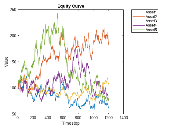
Optimize the Asset Allocation Directly Against Factors with a Problem-Based Definition Framework
For the factors, you can use statistical factors extracted from the asset return series. In this example, you use principal component analysis (PCA) to extract statistical factors [1]. You can then use this factor model to solve the portfolio optimization problem.
With a factor model, p asset returns can be expressed as a linear combination of k factor returns, , where k<<p. In the mean-variance framework, portfolio risk is
, with ,
where:
is the portfolio return (a scalar).
is the asset return.
is the mean of asset return.
is the factor loading, with the dimensions p-by-k.
is the factor return.
is the idiosyncratic return related to each asset.
is the asset weight.
is the factor weight.
is the covariance of factor returns.
is the variance of idiosyncratic returns.
The parameters , , , are p-by-1 column vectors, and are k-by-1 column vectors, is a p-by-p matrix, is a k-by-k matrix, and is a p-by-p diagonal matrix.
Therefore, the mean-variance optimization problem is formulated as
, ,.
In the p dimensional space formed by p asset returns, PCA finds the most important k directions that capture the most important variations in the given returns of p assets. Usually, k is less than p. Therefore, by using PCA you can decompose the p asset returns into the k factors, which greatly reduces the dimension of the problem. The k principal directions are interpreted as factor loadings and the scores from the decomposition are interpreted as factor returns. For more information, see pca (Statistics and Machine Learning Toolbox™). In this example, use k = 10 as the number of principal components. Alternatively, you can also find the k value by defining a threshold for the total variance represented as the top k principal components. Usually 95% is an acceptable threshold.
k = 10;
[factorLoading,factorRetn,latent,tsq,explained,mu] = pca(stockReturns{training,:}, 'NumComponents', k);
disp(size(factorLoading))
100 10
disp(size(factorRetn))
1200 10
In the output p-by-k factorLoading, each column is a principal component. The asset return vector at each timestep is decomposed to these k dimensional spaces, where k << p. The output factorRetn is a trainingNum-by-k dimension.
Alternatively, you can also use the covarianceDenoising function to estimate a covariance matrix (denoisedCov) using denoising to reduce the noise and enhance the signal of the empirical covariance matrix. [1] The goal of denoising is to separate the eigenvalues associated with signal from the ones associated with noise and shrink the eigenvalues associated with noise to enhance the signal. Thus, covarianceDenoising is a reasonable tool to identify the number of factors.
[denoisedCov,numFactorsDenoising] = covarianceDenoising(stockReturns{training,:});The number of factors (numFactorsDenoising) is 6.
disp(numFactorsDenoising)
6
Estimate the factor covariance matrix with factor returns (factorRetn) obtained using the pca function.
covarFactor = cov(factorRetn);
You can reconstruct the p asset returns for each observation using each k factor returns by following .
Reconstruct the total 1200 observations for the training set.
reconReturn = factorRetn*factorLoading' + mu;
unexplainedRetn = stockReturns{training,:} - reconReturn;
There are unexplained asset returns because the remaining (p - k) principal components are dropped. You can attribute the unexplained asset returns to the asset-specific risks represented as D.
unexplainedCovar = diag(cov(unexplainedRetn));
D = diag(unexplainedCovar);
You can use a problem-based definition framework from Optimization Toolbox™ to construct the variables, objective, and constraints for the problem: , ,. The problem-based definition framework enables you to define variables and express objective and constraints symbolically. You can add other constraints or use a different objective based on your specific problem. For more information, see First Choose Problem-Based or Solver-Based Approach.
targetRisk = 0.007;  % Standard deviation of portfolio return
tRisk = targetRisk*targetRisk;  % Variance of portfolio return
meanStockRetn = mean(stockReturns{training,:});

optimProb = optimproblem('Description','Portfolio with factor covariance matrix','ObjectiveSense','max');
wgtAsset = optimvar('asset_weight', p, 1, 'Type', 'continuous', 'LowerBound', 0, 'UpperBound', 1);
wgtFactor = optimvar('factor_weight', k, 1, 'Type', 'continuous');

optimProb.Objective = sum(meanStockRetn'.*wgtAsset);

optimProb.Constraints.asset_factor_weight = factorLoading'*wgtAsset - wgtFactor == 0;
optimProb.Constraints.risk = wgtFactor'*covarFactor*wgtFactor + wgtAsset'*D*wgtAsset <= tRisk;
optimProb.Constraints.budget = sum(wgtAsset) == 1;

x0.asset_weight = ones(p, 1)/p;
x0.factor_weight = zeros(k, 1);
opt = optimoptions("fmincon", "Algorithm","sqp", "Display", "off", ...
    'ConstraintTolerance', 1.0e-8, 'OptimalityTolerance', 1.0e-8, 'StepTolerance', 1.0e-8);
x = solve(optimProb,x0, "Options",opt);
assetWgt1 = x.asset_weight;
In this example, you are maximizing the portfolio return for a target risk. This is a nonlinear programming problem with a quadratic constraint and you use fmincon to solve this problem.
Check for asset allocations that are over 5% to determine which assets have large investment weights.
percentage = 0.05;
AssetName = stockReturns.Properties.VariableNames(assetWgt1>=percentage)';
Weight = assetWgt1(assetWgt1>=percentage);
T1 = table(AssetName, Weight)
T1=7×2 table
     AssetName      Weight
    ___________    ________

    {'Asset9' }    0.080054
    {'Asset32'}     0.22355
    {'Asset47'}     0.11369
    {'Asset57'}    0.088321
    {'Asset61'}    0.068845
    {'Asset75'}    0.063648
    {'Asset94'}     0.22163
Optimize Asset Allocation Using Portfolio Class with Factor Information
If you already have the factor loading and factor covariance matrix from some other analysis or third-party provider, you can use this information to compute the asset covariance matrix and then directly run a mean-variance optimization using the Portfolio class. Recall that portfolio risk is , so you can obtain the covariance of the asset returns by .
Use estimateFrontierByRisk in the Portfolio class to solve the optimization problem: ,. The Portfolio class supports has a variety of built-in constraints that you can use to describe your portfolio problem and estimate the risk and returns on the efficient frontier. For more information, see Supported Constraints for Portfolio Optimization Using Portfolio Objects.
covarAsset = factorLoading*covarFactor*factorLoading'+D;
covarAsset = (covarAsset+covarAsset')/2; % Ensures matrix is symmetric
port = Portfolio("AssetMean", meanStockRetn, 'AssetCovar', covarAsset, 'LowerBound', 0, 'UpperBound', 1, ...
    'Budget', 1);
assetWgt2 = estimateFrontierByRisk(port, targetRisk);

AssetName = stockReturns.Properties.VariableNames(assetWgt2>=percentage)';
Weight = assetWgt2(assetWgt2>=percentage);
T2 = table(AssetName, Weight)
T2=7×2 table
     AssetName      Weight
    ___________    ________

    {'Asset9' }    0.080061
    {'Asset32'}     0.22355
    {'Asset47'}     0.11369
    {'Asset57'}    0.088314
    {'Asset61'}    0.068847
    {'Asset75'}    0.063643
    {'Asset94'}     0.22163
Portfolio Optimization Results
Tables T1 and T2 show an identical allocation for the asset allocations that are over 5%. Therefore, in this example, both approaches to portfolio optimization with a factor model obtain asset weights that are identical.
Visualize the performance of the optimized allocation over the testing period.
retn = stockReturns{test, :}*assetWgt1;
plot(ret2tick(retn, 'method', 'simple')*100); hold off;
xlabel('Timestep');
ylabel('Value');
title('Portfolio Equity Curve');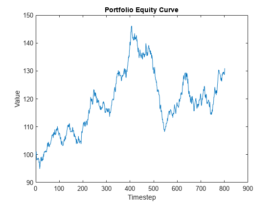
This example demonstrates how to derive statistical factors from asset returns using PCA and then use these factors to perform a factor-based portfolio optimization. This example also shows how to use these statistical factors with the Portfolio class. In practice, you can adapt this example to incorporate some measurable market factors, such as industrial factors or ETF returns from various sectors, to describe the randomness in the market [1]. You can define custom constraints on the weights of factors or assets with high flexibility using the problem-based definition framework from Optimization Toolbox™. Alternatively, you can work directly with the Portfolio class to run a portfolio optimization with various built-in constraints.
Reference
Lòpez de Prado, M. Machine Learning for Asset Managers. Cambridge University Press, 2020.
Meucci, A. "Modeling the Market." Risk and Asset Allocation. Berlin:Springer, 2009.
See Also
Portfolio | setBounds | addGroups | setAssetMoments | estimateAssetMoments | estimateBounds | plotFrontier | estimateFrontierLimits | estimateFrontierByRisk | estimatePortRisk
Topics
- Creating the Portfolio Object
- Working with Portfolio Constraints Using Defaults
- Validate the Portfolio Problem for Portfolio Object
- Estimate Efficient Portfolios for Entire Efficient Frontier for Portfolio Object
- Estimate Efficient Frontiers for Portfolio Object
- Postprocessing Results to Set Up Tradable Portfolios
- Portfolio Optimization with Semicontinuous and Cardinality Constraints
- Black-Litterman Portfolio Optimization Using Financial Toolbox
- Portfolio Optimization Against a Benchmark
- Portfolio Optimization Examples Using Financial Toolbox
- Portfolio Optimization Using Social Performance Measure
- Diversify Portfolios Using Custom Objective
- Portfolio Object
- Portfolio Optimization Theory
- Portfolio Object Workflow