Bayesian Stochastic Search Variable Selection
This example shows how to implement stochastic search variable selection (SSVS), a Bayesian variable selection technique for linear regression models.
Introduction
Consider this Bayesian linear regression model.
The regression coefficients .
.
The disturbances .
The disturbance variance , where is the inverse gamma distribution with shape A and scale B.
The goal of variable selection is to include only those predictors supported by data in the final regression model. One way to do this is to analyze the permutations of models, called regimes, where models differ by the coefficients that are included. If is small, then you can fit all permutations of models to the data, and then compare the models by using performance measures, such as goodness-of-fit (for example, Akaike information criterion) or forecast mean squared error (MSE). However, for even moderate values of , estimating all permutations of models is inefficient.
A Bayesian view of variable selection is a coefficient, being excluded from a model, has a degenerate posterior distribution. That is, the excluded coefficient has a Dirac delta distribution, which has its probability mass concentrated on zero. To circumvent the complexity induced by degenerate variates, the prior for a coefficient being excluded is a Gaussian distribution with a mean of 0 and a small variance, for example . Because the prior is concentrated around zero, the posterior must also be concentrated around zero.
The prior for the coefficient being included can be , where is sufficiently away from zero and is usually zero. This framework implies that the prior of each coefficient is a Gaussian mixture model.
Consider the latent, binary random variables , , such that:
indicates that and that is included in the model.
indicates that and that is excluded from the model.
.
The sample space of has a cardinality of , and each element is a -D vector of zeros or ones.
is a small, positive number and .
Coefficients and , are independent, a priori.
One goal of SSVS is to estimate the posterior regime probabilities , the estimates that determine whether corresponding coefficients should be included in the model. Given , is conditionally independent of the data. Therefore, for , this equation represents the full conditional posterior distribution of the probability that variable k is included in the model:
where is the pdf of the Gaussian distribution with scalar mean and variance .
Econometrics Toolbox™ has two Bayesian linear regression models that specify the prior distributions for SSVS: mixconjugateblm and mixsemiconjugateblm. The framework presented earlier describes the priors of the mixconjugateblm model. The difference between the models is that and are independent, a priori, for mixsemiconjugateblm models. Therefore, the prior variance of is () or ().
After you decide which prior model to use, call bayeslm to create the model and specify hyperparameter values. Supported hyperparameters include:
Intercept, a logical scalar specifying whether to include an intercept in the model.Mu, a (p + 1)-by-2 matrix specifying the prior Gaussian mixture means of . The first column contains the means for the component corresponding to , and the second column contains the means corresponding to . By default, all means are 0, which specifies implementing SSVS.V, a (p + 1)-by-2 matrix specifying the prior Gaussian mixture variance factors (or variances) of . Columns correspond to the columns ofMu. By default, the variance of the first component is10and the variance of the second component is0.1.Correlation, a (p + 1)-by-(p + 1) positive definite matrix specifying the prior correlation matrix of for both components. The default is the identity matrix, which implies that the regression coefficients are uncorrelated, a priori.Probability, a (p + 1)-D vector of prior probabilities of variable inclusion (, k = 0,...,_p_) or a function handle to a custom function. and , , are independent, a priori. However, using a function handle (@functionname), you can supply a custom prior distribution that specifies dependencies between and . For example, you can specify forcing out of the model if is included.
After you create a model, pass it and the data to estimate. The estimate function uses a Gibbs sampler to sample from the full conditionals, and estimate characteristics of the posterior distributions of and . Also, estimate returns posterior estimates of .
For this example, consider creating a predictive linear model for the US unemployment rate. You want a model that generalizes well. In other words, you want to minimize the model complexity by removing all redundant predictors and all predictors that are uncorrelated with the unemployment rate.
Load and Preprocess Data
Load the US macroeconomic data set Data_USEconModel.mat.
load Data_USEconModelThe data set includes the MATLAB® timetable DataTimeTable, which contains 14 variables measured from Q1 1947 through Q1 2009; UNRATE is the US unemployment rate. For more details, enter Description at the command line.
Plot all series in the same figure, but in separate subplots.
figure
tiledlayout(4,4)
for j = 1:size(DataTimeTable,2)
    nexttile
    plot(DataTimeTable.Time,DataTimeTable{:,j});
    title(DataTimeTable.Properties.VariableNames(j));
end
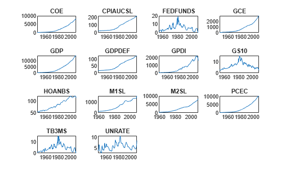
All series except FEDFUNDS, GS10, TB3MS, and UNRATE appear to have an exponential trend.
Apply the log transform to those variables with an exponential trend.
hasexpotrend = ~ismember(DataTimeTable.Properties.VariableNames,...
    ["FEDFUNDS" "GD10" "TB3MS" "UNRATE"]);
DataTimeTableLog = varfun(@log,DataTimeTable,'InputVariables',...
    DataTimeTable.Properties.VariableNames(hasexpotrend));
DataTimeTableLog = [DataTimeTableLog ...
    DataTimeTable(:,DataTimeTable.Properties.VariableNames(~hasexpotrend))];
DataTimeTableLog is a timetable like DataTimeTable, but those variables with an exponential trend are on the log scale.
Coefficients that have relatively large magnitudes tend to dominate the penalty in the lasso regression objective function. Therefore, it is important that variables have a similar scale when you implement lasso regression. Compare the scales of the variables in DataTimeTableLog by plotting their box plots on the same axis.
figure;
boxplot(DataTimeTableLog.Variables,'Labels',DataTimeTableLog.Properties.VariableNames);
h = gcf;
h.Position(3) = h.Position(3)*2.5;
title('Variable Box Plots');
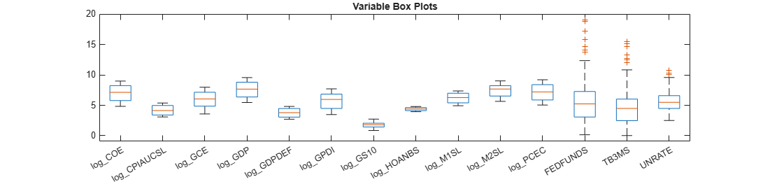
The variables have fairly similar scales.
To tune the prior Gaussian mixture variance factors, follow this procedure:
Partition the data into estimation and forecast samples.
Fit the models to the estimation sample and specify, for all , and .
Use the fitted models to forecast responses into the forecast horizon.
Estimate the forecast MSE for each model.
Choose the model with the lowest forecast MSE.
George and McCulloch suggest another way to tune the prior variances of in [1].
Create estimation and forecast sample variables for the response and predictor data. Specify a forecast horizon of 4 years (16 quarters).
fh = 16;
y = DataTimeTableLog.UNRATE(1:(end - fh));
yF = DataTimeTableLog.UNRATE((end - fh + 1):end);
isresponse = DataTimeTable.Properties.VariableNames == "UNRATE";
X = DataTimeTableLog{1:(end - fh),~isresponse};
XF = DataTimeTableLog{(end - fh + 1):end,~isresponse};
p = size(X,2); % Number of predictors
predictornames = DataTimeTableLog.Properties.VariableNames(~isresponse);
Create Prior Bayesian Linear Regression Models
Create prior Bayesian linear regression models for SSVS by calling bayeslm and specifying the number of predictors, model type, predictor names, and component variance factors. Assume that and are dependent, a priori (mixconjugateblm model).
V1 = [10 50 100];
V2 = [0.05 0.1 0.5];
numv1 = numel(V1);
numv2 = numel(V2);

PriorMdl = cell(numv1,numv2); % Preallocate

for k = 1:numv2
    for j = 1:numv1
        V = [V1(j)*ones(p + 1,1) V2(k)*ones(p + 1,1)];
        PriorMdl{j,k} = bayeslm(p,'ModelType','mixconjugateblm',...
            'VarNames',predictornames,'V',V);
    end
end
PriorMdl is a 3-by-3 cell array, and each cell contains a mixconjugateblm model object.
Plot the prior distribution of log_GDP for the models in which V2 is 0.5.
for j = 1:numv1
    [~,~,~,h] = plot(PriorMdl{j,3},'VarNames',"log_GDP");
    title(sprintf("Log GDP, V1 = %g, V2 = %g",V1(j),V2(3)));
    h.Tag = strcat("fig",num2str(V1(j)),num2str(V2(3)));
end
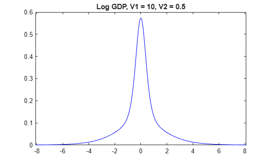
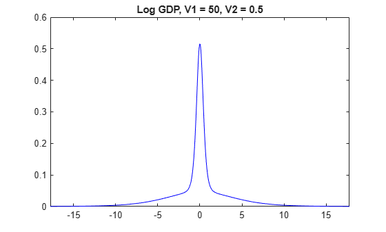
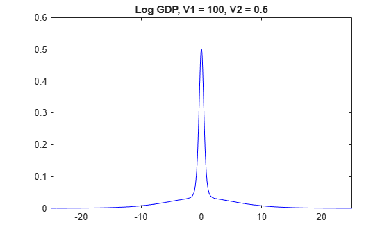
The prior distributions of have the spike-and-slab shape. When V1 is low, more of the distribution is concentrated around 0, which makes it more difficult for the algorithm to attribute a high value for beta. However, variables the algorithm identifies as important are regularized, in that the algorithm does not attribute a high magnitude to the corresponding coefficients.
When V1 is high, more density occurs well away from zero, which makes it easier for the algorithm to attribute non-zero coefficients to important predictors. However, if V1 is too high, then important predictors can have inflated coefficients.
Perform SSVS Variable Selection
To perform SSVS, estimate the posterior distributions by using estimate. Use the default options for the Gibbs sampler.
PosteriorMdl = cell(numv1,numv2);
PosteriorSummary = cell(numv1,numv2);

rng(1); % For reproducibility
for k = 1:numv2
    for j = 1:numv1
        [PosteriorMdl{j,k},PosteriorSummary{j,k}] = estimate(PriorMdl{j,k},X,y,...
            'Display',false);
    end
end
Each cell in PosteriorMdl contains an empiricalblm model object storing the full conditional posterior draws from the Gibbs sampler. Each cell in PosteriorSummary contains a table of posterior estimates. The Regime table variable represents the posterior probability of variable inclusion ().
Display a table of posterior estimates of .
RegimeTbl = table(zeros(p + 2,1),'RowNames',PosteriorSummary{1}.Properties.RowNames);
for k = 1:numv2
    for j = 1:numv1
        vname = strcat("V1_",num2str(V1(j)),"__","V2_",num2str(V2(k)));
        vname = replace(vname,".","p");
        tmp = table(PosteriorSummary{j,k}.Regime,'VariableNames',vname);
        RegimeTbl = [RegimeTbl tmp];
    end
end
RegimeTbl.Var1 = [];
RegimeTbl
RegimeTbl=15×9 table
                    V1_10__V2_0p05    V1_50__V2_0p05    V1_100__V2_0p05    V1_10__V2_0p1    V1_50__V2_0p1    V1_100__V2_0p1    V1_10__V2_0p5    V1_50__V2_0p5    V1_100__V2_0p5
                    ______________    ______________    _______________    _____________    _____________    ______________    _____________    _____________    ______________

    Intercept           0.9692                 1                 1            0.9501                1                 1           0.9487           0.9999                 1
    log_COE             0.4686            0.4586            0.5102            0.4487           0.3919            0.4785           0.4575           0.4147            0.4284
    log_CPIAUCSL        0.9713            0.3713            0.4088             0.971           0.3698            0.3856            0.962           0.3714            0.3456
    log_GCE             0.9999                 1                 1            0.9978                1                 1           0.9959                1                 1
    log_GDP             0.7895            0.9921            0.9982            0.7859           0.9959                 1           0.7908           0.9975            0.9999
    log_GDPDEF          0.9977                 1                 1                 1                1                 1           0.9996                1                 1
    log_GPDI                 1                 1                 1                 1                1                 1                1                1                 1
    log_GS10                 1                 1            0.9991                 1                1            0.9992                1           0.9992             0.994
    log_HOANBS          0.9996                 1                 1            0.9887                1                 1           0.9763                1                 1
    log_M1SL                 1                 1                 1                 1                1                 1                1                1                 1
    log_M2SL            0.9989            0.9993            0.9913            0.9996           0.9998            0.9754           0.9951           0.9983            0.9856
    log_PCEC            0.4457            0.6366            0.8421            0.4435           0.6226            0.8342           0.4614            0.624              0.85
    FEDFUNDS            0.0762            0.0386            0.0237            0.0951           0.0465            0.0343           0.1856           0.0953             0.068
    TB3MS               0.2473            0.1788            0.1467            0.2014           0.1338            0.1095           0.2234           0.1185            0.0909
    Sigma2                 NaN               NaN               NaN               NaN              NaN               NaN              NaN              NaN               NaN
Using an arbitrary threshold of 0.10, all models agree that FEDFUNDS is an insignificant or redundant predictor. When V1 is high, TB3MS borders on being insignificant.
Forecast responses and compute forecast MSEs using the estimated models.
yhat = zeros(fh,numv1*numv2);
fmse = zeros(numv1,numv2);

for k = 1:numv2
    for j = 1:numv1
        idx = ((k - 1)*numv1 + j);
        yhat(:,idx) = forecast(PosteriorMdl{j,k},XF);
        fmse(j,k) = sqrt(mean((yF - yhat(:,idx)).^2));
    end
end
Identify the variance factor settings that yield the minimum forecast MSE.
minfmse = min(fmse,[],'all');
[idxminr,idxminc] = find(abs(minfmse - fmse) < eps);
bestv1 = V1(idxminr)
bestv1 = 100
bestv2 = V2(idxminc)
bestv2 =
0.0500
Estimate an SSVS model using the entire data set and the variance factor settings that yield the minimum forecast MSE.
XFull = [X; XF];
yFull = [y; yF];
EstMdl = estimate(PriorMdl{idxminr,idxminc},XFull,yFull);
Method: MCMC sampling with 10000 draws
Number of observations: 201
Number of predictors: 14
| Mean Std CI95 Positive Distribution Regime
-------------------------------------------------------------------------------------
Intercept | 29.3742 4.2707 [20.958, 37.744] 1.000 Empirical 1
log_COE | 3.2471 3.0311 [-0.219, 9.212] 0.834 Empirical 0.6872
log_CPIAUCSL | -0.6306 1.7446 [-5.487, 2.065] 0.399 Empirical 0.3738
log_GCE | -9.4570 1.4537 [-12.283, -6.606] 0.000 Empirical 1
log_GDP | 16.6570 3.7641 [ 9.251, 23.881] 1.000 Empirical 1
log_GDPDEF | 12.9291 2.3326 [ 9.132, 18.785] 1.000 Empirical 1
log_GPDI | -5.9586 0.6224 [-7.160, -4.742] 0.000 Empirical 1
log_GS10 | 1.4715 0.3757 [ 0.720, 2.185] 1.000 Empirical 0.9928
log_HOANBS | -16.0584 1.5243 [-19.048, -13.050] 0.000 Empirical 1
log_M1SL | -4.6445 0.6774 [-5.976, -3.317] 0.000 Empirical 1
log_M2SL | 5.3836 1.2781 [ 2.854, 7.886] 1.000 Empirical 0.9993
log_PCEC | -9.6984 3.4191 [-16.079, -1.726] 0.010 Empirical 0.9802
FEDFUNDS | -0.0161 0.0562 [-0.123, 0.096] 0.377 Empirical 0.0261
TB3MS | -0.1448 0.0751 [-0.297, 0.000] 0.025 Empirical 0.0727
Sigma2 | 0.2889 0.0288 [ 0.238, 0.351] 1.000 Empirical NaN
EstMdl is an empiricalblm model representing the result of performing SSVS. You can use EstMdl to forecast the unemployment rate given future predictor data , for example.
References
[1] George, E. I., and R. E. McCulloch. "Variable Selection Via Gibbs Sampling." Journal of the American Statistical Association. Vol. 88, No. 423, 1993, pp. 881–889.