Detect Anomalies in Signals Using deepSignalAnomalyDetector
This example shows how to detect anomalies in signals using deepSignalAnomalyDetector (Signal Processing Toolbox). The deepSignalAnomalyDetector object implements autoencoder architectures that can be trained using semi-supervised or unsupervised learning. The detector can find abnormal points or regions, or identify whole signals as anomalous. The object also provides several convenient functions that you can use to visualize and analyze results.
Anomalies are data points that deviate from the overall pattern of an entire data set. Detecting anomalies in time-series data has broad applications in domains such as manufacturing, predictive maintenance, and human health monitoring. In many scenarios, manually labeling an entire data set to train a model to detect anomalies is unrealistic, especially when the relevant data has many more normal samples than abnormal ones. In those scenarios, anomaly detection based on semi-supervised or unsupervised learning is a more viable solution.
deepSignalAnomalyDetector provides two types of autoencoder architecture. An autoencoder is a deep neural network that is trained to replicate the input data at its output such that the reconstruction error is as small as possible. The data used to train the autoencoder can consist exclusively of normal samples or can include a small percentage of samples with anomalies. The data does not have to be labeled. After you train the autoencoder, it can reconstruct test data, compute the reconstruction error for each sample, and declare as anomalies those samples whose reconstruction error surpasses a specified threshold.
Case 1: Detect Abnormal Heartbeat Sequences
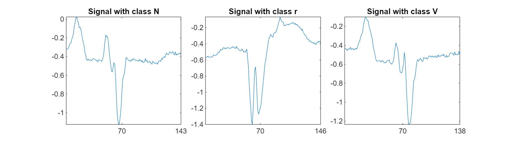
This section uses the deepSignalAnomalyDetector object to detect abnormal heartbeat sequences in data from the BIDMC Congestive Heart Failure Database [1]. The heartbeat collection has 5405 electrocardiogram (ECG) sequences of varying length, each sampled at 250 Hz and containing three categories of heartbeat:
N — Normal
r — R-onT premature ventricular contraction
V — Premature ventricular contraction
The data is labeled, but in this example you use the labels only for testing and performance evaluation. The autoencoder training process is fully unsupervised.
Load Data
Download the heartbeat data from https://ssd.mathworks.com/supportfiles/SPT/data/PhysionetBIDMC.zip using the downloadSupportFile function. The whole data set is approximately 2 MB in size. The ecgSignals contains signals and ecgLabels contains labels.
datasetZipFile = matlab.internal.examples.downloadSupportFile('SPT','data/PhysionetBIDMC.zip');
datasetFolder = fullfile(fileparts(datasetZipFile),'PhysionetBDMC');
if ~exist(datasetFolder,'dir')
    unzip(datasetZipFile,datasetFolder);
end
ds1 = load(fullfile(datasetFolder,"chf07.mat"));
ecgSignals1 = ds1.ecgSignals
ecgSignals1=5405×1 cell array
    146×1 double
    140×1 double
    139×1 double
    143×1 double
    143×1 double
    145×1 double
    147×1 double
    139×1 double
    143×1 double
    139×1 double
    146×1 double
    143×1 double
    144×1 double
    142×1 double
      ⋮
ecgLabels1 = ds1.ecgLabels;
cnts = countlabels(ecgLabels1)
cnts=3×3 table
    N    5288    97.8353
    V       6     0.1110
    r     111     2.0537
Visualize typical waveforms corresponding to each of the three heartbeat categories.
helperPlotECG(ecgSignals1,ecgLabels1)
Get the indices corresponding to each category and split the data set into training and testing sets. In the training set, include 60% of samples to maintain the natural anomaly distribution. Exclude class V samples from the training set but include them in the test set. Including these samples in the test set determines whether the autoencoder can detect previously unobserved anomaly types.
idxN = find(strcmp(ecgLabels1,"N"));
idxR = find(strcmp(ecgLabels1,"r"));
idxV = find(strcmp(ecgLabels1,"V"));
idxs = splitlabels(ecgLabels1,0.6,Exclude="V");
idxTrain = [idxs{1}];
idxTest = [idxs{2};idxV];
countlabels(ecgLabels1(idxTrain))
ans=2×3 table
    N    3173    97.9321
    r      67     2.0679
countlabels(ecgLabels1(idxTest))
ans=3×3 table
    N    2115    97.6905
    V       6     0.2771
    r      44     2.0323
Create and Train Detector
Create a deepSignalAnomalyDetector object with a long short-term memory (LSTM) model. Set WindowLength to "fullSignal" to determine whether each complete signal segment is normal or abnormal.
DLSTM1 = deepSignalAnomalyDetector(1,"lstm",WindowLength="fullSignal")
DLSTM1 =
  deepSignalAnomalyDetectorLSTM with properties:

                IsTrained: 0
              NumChannels: 1

   Model Information
                ModelType: 'lstmautoencoder'
       EncoderHiddenUnits: [32 16]
       DecoderHiddenUnits: [16 32]

   Threshold Information
                Threshold: []
          ThresholdMethod: 'contaminationFraction'
       ThresholdParameter: 0.0100

   Window Information
             WindowLength: 'fullSignal'
    WindowLossAggregation: 'mean'
Train the detector using the adaptive moment estimation (Adam) optimizer, which is one of the most popular solvers for deep learning training. The maximum number of epochs often needs to be adjusted according to the data set size and training process. Because the number of samples is large, set MaxEpochs to 200.
opts = trainingOptions("adam", ...
    MaxEpochs=200, ...
    MiniBatchSize=500);
trainDetector(DLSTM1,ecgSignals1(idxTrain),opts);
    Iteration    Epoch    TimeElapsed    LearnRate    TrainingLoss
    _________    _____    ___________    _________    ____________
            1        1       00:00:01        0.001         0.22301
           50        9       00:00:15        0.001        0.043575
          100       17       00:00:30        0.001        0.036187
          150       25       00:00:44        0.001         0.03203
          200       34       00:00:59        0.001        0.027874
          250       42       00:01:13        0.001        0.026719
          300       50       00:01:27        0.001         0.02708
          350       59       00:01:42        0.001        0.026182
          400       67       00:01:56        0.001        0.025803
          450       75       00:02:10        0.001        0.026763
          500       84       00:02:25        0.001        0.025313
          550       92       00:02:39        0.001        0.023865
          600      100       00:02:53        0.001        0.020967
          650      109       00:03:08        0.001        0.015418
          700      117       00:03:22        0.001        0.010735
          750      125       00:03:36        0.001       0.0090826
          800      134       00:03:51        0.001       0.0074879
          850      142       00:04:05        0.001       0.0076077
          900      150       00:04:19        0.001       0.0081417
          950      159       00:04:34        0.001       0.0070189
         1000      167       00:04:48        0.001       0.0074735
         1050      175       00:05:02        0.001       0.0077058
         1100      184       00:05:17        0.001       0.0064108
         1150      192       00:05:31        0.001       0.0068832
         1200      200       00:05:45        0.001       0.0074522
Training stopped: Max epochs completed
Computing threshold...
Threshold computation completed.
Adjust Threshold
By default, the deepSignalAnomalyDetector object computes the threshold assuming that 1% of the data in the training set are abnormal. This assumption is not always true, so you often need to adjust the threshold by changing the automatic threshold method or by setting the threshold value manually.
Use the plotLoss (Signal Processing Toolbox) function to visualize the losses of the training set and the current threshold value. Each stem corresponds to the reconstruction error for one of the signals in the training data set.
figure
plotLoss(DLSTM1,ecgSignals1(idxTrain))
ylim([0,0.1])
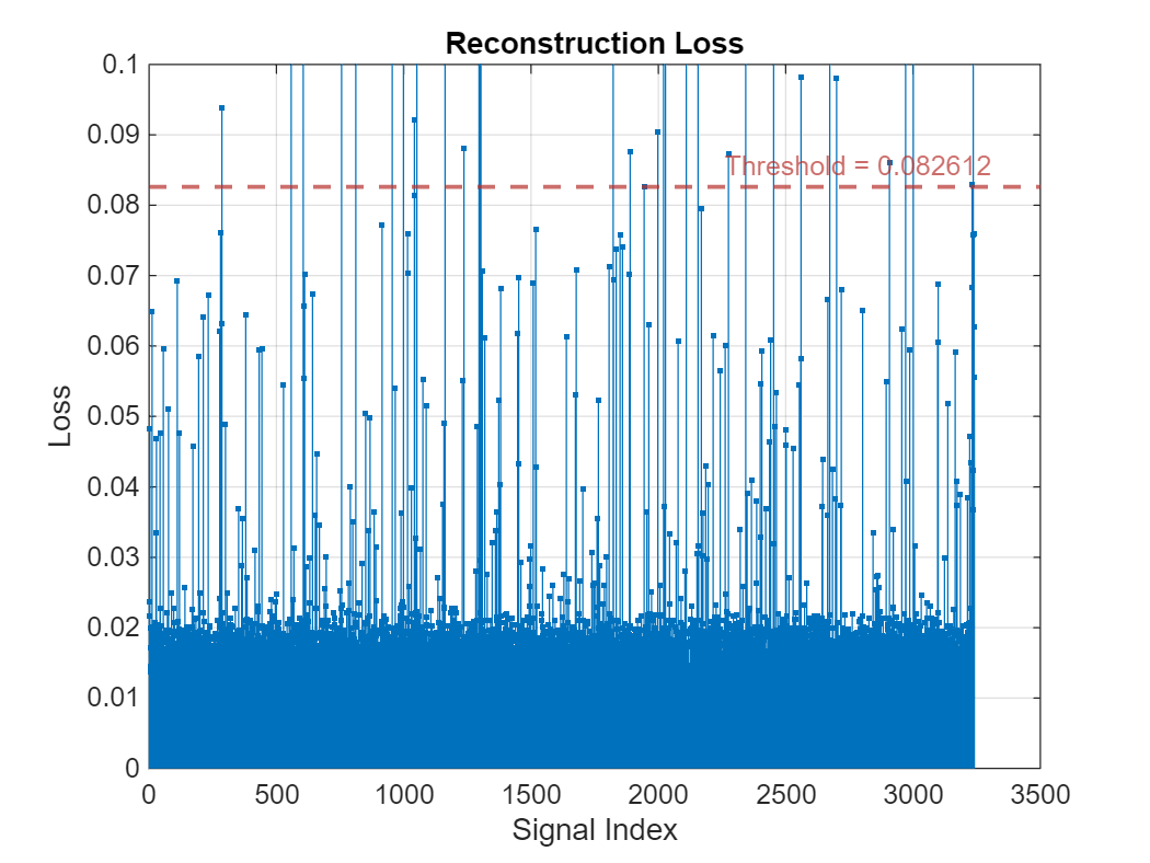
Based on the plotLoss output, set threshold value manually such that the few sporadic losses that exceed the threshold are most likely anomalies.
updateDetector(DLSTM1, ...
    ThresholdMethod="Manual", ...
    Threshold=0.03)
To validate the choice of threshold, plot the distribution of the reconstruction errors for the normal and the abnormal data using plotLossDistribution (Signal Processing Toolbox). The histogram to the left of the threshold corresponds to the distribution of normal data. The histogram to the right of the threshold corresponds to the distribution of abnormal data. The chosen threshold value successfully separates the normal and abnormal groups.
% ecgSignals1(idxN) contains normal signals only
% ecgSignals1([idxR;idxV]) contains abnormal signals
plotLossDistribution(DLSTM1,ecgSignals1(idxN),ecgSignals1([idxR; idxV]))

Detect Anomalies and Evaluate Performance
Pick one sample from each category in the testing set and plot the reconstructed signal using plotAnomalies (Signal Processing Toolbox). The red lines represent signals the detector classifies as abnormal. A good sign that the detector is successfully trained is that it can adequately reconstruct normal signals and cannot adequately reconstruct abnormal signals.
figure(Position=[0 0 500 300])
idxNTest = intersect(idxN,idxTest); % Class N
plotAnomalies(DLSTM1,ecgSignals1(idxNTest(1)),PlotReconstruction=true)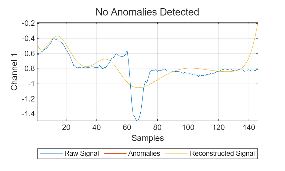
figure(Position=[0 0 500 300])
idxVTest = intersect(idxV,idxTest); % Class V
plotAnomalies(DLSTM1,ecgSignals1(idxVTest(1)),PlotReconstruction=true)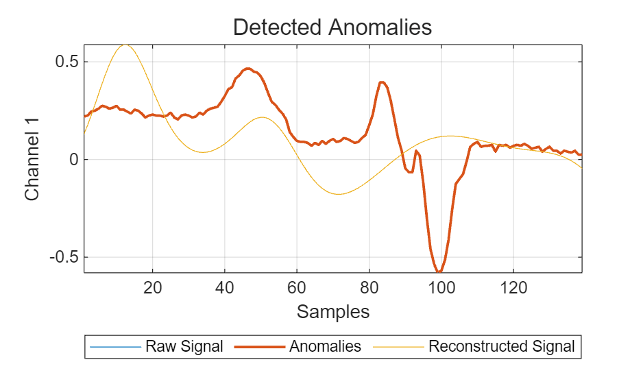
figure(Position=[0 0 500 300])
idxRTest = intersect(idxR,idxTest); % Class r
plotAnomalies(DLSTM1,ecgSignals1(idxRTest(1)),PlotReconstruction=true)
Use the detect (Signal Processing Toolbox) object function of the detector with both training and testing sets to detect anomalies and compute reconstruction losses.
[labelsTrainPred1,lossTrainPred1] = detect(DLSTM1,ecgSignals1(idxTrain));
[labelsTestPred1,lossTestPred1] = detect(DLSTM1,ecgSignals1(idxTest));
There are two different anomaly detection tasks.
Detect anomalies contained in the training set, also known as outlier detection.
Detect anomalies in new observations outside the training set, also known as novelty detection.
Analyze the performance of the trained autoencoder in the two tasks.
You can use a receiver operating characteristic (ROC) curve to evaluate the accuracy of a detector over a range of decision thresholds. The area under the ROC curve (AUC) measures the overall performance. The closer the AUC is to 1, the stronger the detection ability of the detector. Compute the AUC using the rocmetrics function. The AUC is close to one for the outlier detection, and slightly smaller but still very good for the novelty detection.
figure("Position",[0 0 600 300])
tiledlayout(1,2,TileSpacing="compact")
nexttile
rocc = rocmetrics(ecgLabels1(idxTrain)~="N",cell2mat(lossTrainPred1),true);
plot(rocc,ShowModelOperatingPoint=false)
title(["Training Set ROC Curve","(Outlier Detection)"])
nexttile
rocc = rocmetrics(ecgLabels1(idxTest)~="N",cell2mat(lossTestPred1),true);
plot(rocc,ShowModelOperatingPoint=false)
title(["Testing Set ROC Curve","(Novelty Detection)"])

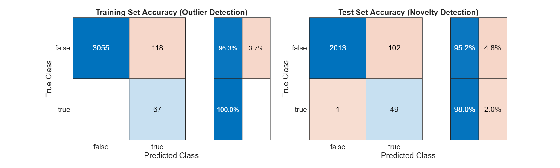
Compute the detection accuracy with the previously specified threshold.
figure("Position",[0 0 1000 300])
tiledlayout(1,2,TileSpacing="compact")
nexttile
cm = confusionchart(ecgLabels1(idxTrain)~="N",cell2mat(labelsTrainPred1));
cm.RowSummary = "row-normalized";
title("Training Set Accuracy (Outlier Detection)")
nexttile
cm = confusionchart(ecgLabels1(idxTest)~="N",cell2mat(labelsTestPred1));
cm.RowSummary = "row-normalized";
title("Test Set Accuracy (Novelty Detection)")
Case 2: Detect Anomalous Points in Continuous Long Time Series
The previous section showed how to detect anomalies in data sets containing multiple signal segments and determine whether each segment was abnormal or not. In this section the data set is a single signal. The goal is to detect anomalies in the signal and the times at which they occur.
Use a deepSignalAnomalyDetector on a long ECG recording to detect anomalies caused by ventricular tachycardia. The data is from the Sudden Cardiac Death Holter Database [2]. The ECG signal has a sampling rate of 250 Hz.
Download and Prepare Data
Download the data from https://ssd.mathworks.com/supportfiles/SPT/data/PhysionetSDDB.zip using the downloadSupportFile function. The data set contains two timetables. The timetable X contains the ECG signal. Timetable Y contains labels that indicate whether each sample of the ECG signal is normal. As in the previous section, you use the labels only to verify the accuracy of the detector.
datasetZipFile = matlab.internal.examples.downloadSupportFile('SPT','data/PhysionetSDDB.zip');
datasetFolder = fullfile(fileparts(datasetZipFile),'PhysionetSDDB');
if ~exist(datasetFolder,'dir')
    unzip(datasetZipFile,datasetFolder);
end
ds2 = load(fullfile(datasetFolder,"sddb49.mat"));
ecgSignals2 = ds2.X;
ecgLabels2 = ds2.y;
Normalize the full signal and visualize it. Overlay the located anomalies. The anomaly detection in this case is challenging because, as often happens in ECG recordings, the signal baseline drifts. These changes in baseline level can easily be misclassified as anomalies.
A common approach to choose training data is to use a segment of the signal where it is evident that there are no anomalies. In many situations, the beginning of a recording is usually normal, such as in this ECG signal. Choose the first 200 seconds of the recording to train the model with purely normal data. Use the rest of the recording to test the performance of the anomaly detector. The training data contain segments with baseline drift, ideally, the detector learns and adapts to this pattern and considers it normal.
dataProcessed = normalize(ecgSignals2);
figure
plot(dataProcessed.Time,dataProcessed.Variables)
hold on
plot(dataProcessed(ecgLabels2.anomaly,:).Time,dataProcessed(ecgLabels2.anomaly,:).Variables,".")
hold off
xlabel("Time (s)")
ylabel("Normalized ECG Amplitude")
title("sddb49 ECG Signal")
legend(["Signal" "Anomaly"])

Split the data set into training and testing sets.
fs = 250;
idxTrain2 = 1:200*fs;
idxTest2 =idxTrain2(end)+1:height(dataProcessed);
dataProcessedTrain = dataProcessed(idxTrain2,:);
labelsTrainTrue = ecgLabels2(idxTrain2,:);
dataProcessedTest = dataProcessed(idxTest2,:);
labelsTestTrue = ecgLabels2(idxTest2,:);
Create and Train Detector
Create a deepSignalAnomalyDetector with a convolutional autoencoder model.
The training set contains only normal data. So, it is reasonable to use the maximum reconstruction error as a threshold when declaring a signal segment to be an anomaly. Set the ThresholdMethod property to "max". To incorporate the complexity of the signal due to baseline drift, use a larger network than the default. To detect anomalies over each sample of the signal, keep the window length to its default value of one sample.
DCONV2 = deepSignalAnomalyDetector(1,"conv", ...
    FilterSize=32, ...
    NumFilters=16, ...
    NumDownsampleLayers=4, ...
    ThresholdMethod="max")
DCONV2 =
  deepSignalAnomalyDetectorCNN with properties:

                IsTrained: 0
              NumChannels: 1

   Model Information
                ModelType: 'convautoencoder'
               FilterSize: 32
               NumFilters: 16
      NumDownsampleLayers: 4
         DownsampleFactor: 2
       DropoutProbability: 0.2000

   Threshold Information
                Threshold: []
          ThresholdMethod: 'max'
       ThresholdParameter: 1

   Window Information
             WindowLength: 1
            OverlapLength: 'auto'
    WindowLossAggregation: 'mean'
To ensure full training of the large network, set the maximum number of epochs to 500. To plot training progress during training instead of presenting it in a table, set the Plots training option to "training-progress" and Verbose to false.
opts = trainingOptions("adam",MaxEpochs=500,Plots="training-progress",Verbose=false);
trainDetector(DCONV2,dataProcessedTrain,opts)

Detect Anomalies and Evaluate Performance
Plot the reconstruction error distribution of the test signal and compare it to ground truth labels. There is an obvious high loss peak corresponds to the location of an anomaly. The distribution also contains multiple smaller fluctuations.
figure
tiledlayout(2,1)
nexttile
plotLoss(DCONV2,dataProcessed(idxTest2,:));
nexttile
stem(ecgLabels2{idxTest2,:},".")
grid on
yticks([0 1])
yticklabels({"Normal","Abnormal"})
title("Ground Truth Labels")
xlabel("Window Index")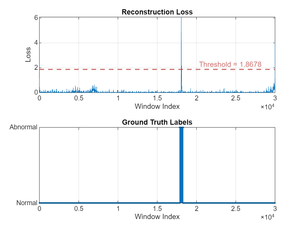
View the signal reconstruction in a region of the test set with abnormal heartbeats and in a region of the test set with baseline drift. The reconstructed signal follows the baseline very well and deviates from the original signal only at anomaly points.
plotAnomalies(DCONV2,dataProcessed(250*fs:300*fs,:),PlotReconstruction=true)
title("Test Region with Abnormal Heartbeats")
grid on

plotAnomalies(DCONV2,dataProcessed(210*fs:250*fs,:),PlotReconstruction=true)
title("Test Region with Baseline Drift")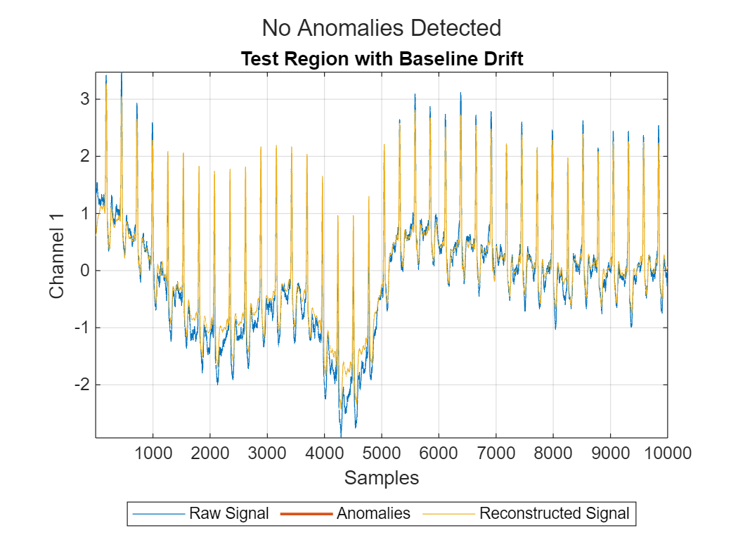
Case 3: Detect Anomalous Regions in Multichannel Signals
There are scenarios where the data contains multiple signals coming from different measurements. These signals can include acceleration, temperature, and the rotational speed of a motor. You can train the deepSignalAnomalyDetector object with multivariate signals and detect anomalies in these multi-measurement observations.
Load and Prepare Data
Load the waveform data set WaveformData. The observations are arrays of size numChannels-by-numTimeSteps, where numChannels is the number of channels and numTimeSteps is the number of time steps in the sequence. Transpose the arrays so that the columns correspond to the time steps. Display the first few cells of the data.
load WaveformData
head(data)
{103×3 double}
{136×3 double}
{140×3 double}
{124×3 double}
{127×3 double}
{200×3 double}
{141×3 double}
{151×3 double}
Visualize the first few sequences in a plot.
numChannels = size(data{1},2);
tiledlayout(2,2)
for ii = 1:4
    nexttile
    stackedplot(data{ii},DisplayLabels="Channel " + (1:numChannels));
    title("Observation " + ii)
    xlabel("Time Step")
end
Partition the data into training and test partitions. Use 90% of the data for training and 10% for testing.
numObservations = numel(data);
rng default
[idxTrain3,~,idxTest3] = dividerand(numObservations,0.9,0,0.1);
signalTrain3 = data(idxTrain3);
signalTest3 = data(idxTest3);
Create and Train Detector
Create a default anomaly detector and specify the number of channels as 3.
DCONV3 = deepSignalAnomalyDetector(3,'lstmf',WindowLen = 5);
trainDetector(DCONV3,signalTrain3)
Iteration Epoch TimeElapsed LearnRate TrainingLoss
_________ _____ ___________ _________ ____________
1 1 00:00:00 0.001 1.3893
50 8 00:00:04 0.001 0.83859
100 15 00:00:07 0.001 0.54641
150 22 00:00:11 0.001 0.44731
200 29 00:00:15 0.001 0.41617
210 30 00:00:16 0.001 0.40876
Training stopped: Max epochs completed
Computing threshold...
Threshold computation completed.
Detect Anomalies and Evaluate Performance
To test the detector, select 50 data sequences at random and add artificial anomalies to them. Randomly select 50 of the sequences to modify.
signalTest3New = signalTest3;
numAnomalousSequences = 50;
rng default
idx = randperm(numel(signalTest3),numAnomalousSequences);
Select a 20-sample region in a random channel of each chosen sequence and replace it with five times the absolute value of its amplitude.
for ii = 1:numAnomalousSequences
    X = signalTest3New{idx(ii)};
    idxPatch = 40:60;
    nch = randi(3);
    OldRegion = X(idxPatch,nch);
    newRegion = 5*abs(OldRegion);
    X(idxPatch,nch) = newRegion;
    signalTest3New{idx(ii)} = X;
end
Use the anomaly detector to find the anomalous regions. Visualize the results for two of the signals. The detector determines that an anomaly exists in a signal when any of its channels shows abnormal behavior.
figure
plotAnomalies(DCONV3,signalTest3New{idx(2)})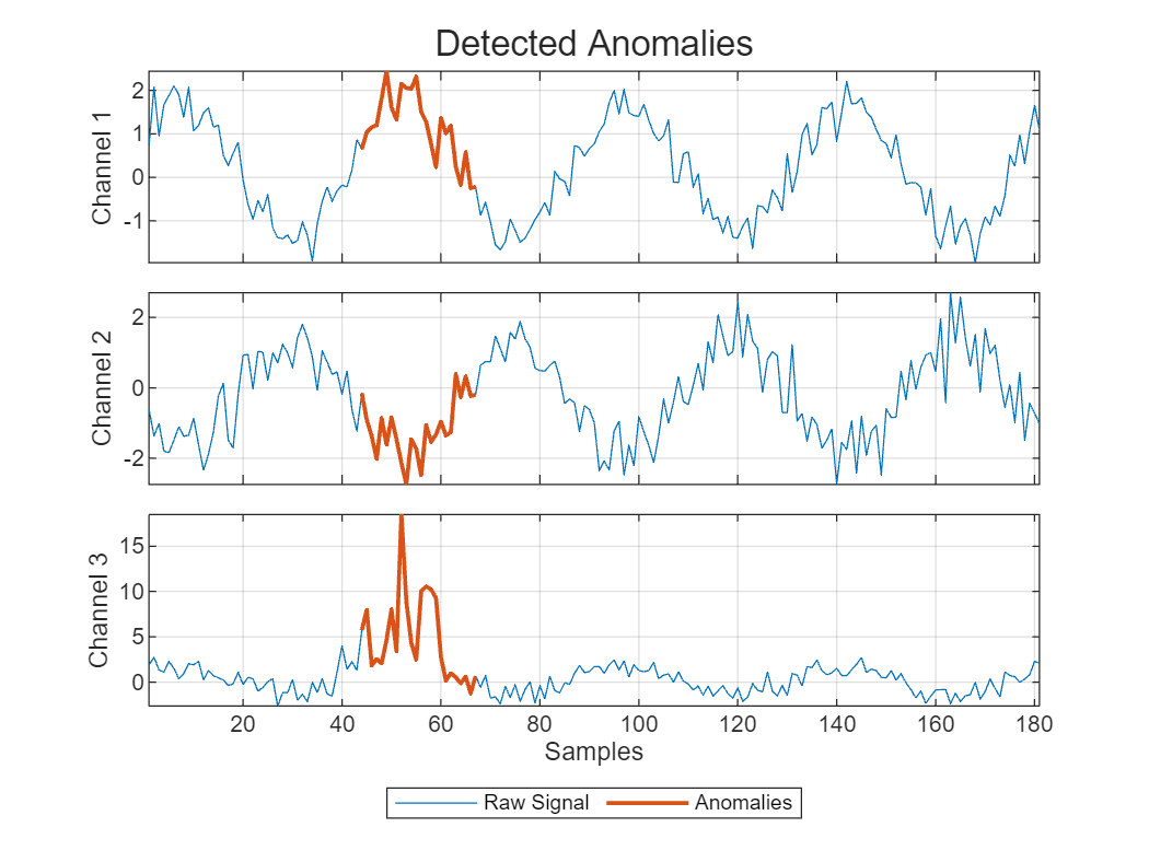
figure
plotAnomalies(DCONV3,signalTest3New{idx(20)})
Conclusion
This example shows how to use a deepSignalAnomalyDetector object trained without labels to detect point, region, or observation anomalies in signal segments, long signals, and multivariate signals.
References
[1] Donald S. Baim, Wilson S. Colucci, E. Scott Monrad, Harton S. Smith, Richard F. Wright, Alyce Lanoue, Diane F. Gauthier, Bernard J. Ransil, William Grossman W, and Eugene Braunwald. “Survival of Patients with Severe Congestive Heart Failure Treated with Oral Milrinone.” Journal of the American College of Cardiology, vol. 7, no. 3, (March 1986): 661–70. https://doi.org/10.1016/S0735-1097(86)80478-8.
[2] Greenwald, Scott David. "Development and analysis of a ventricular fibrillation detector." (M.S. thesis, MIT Dept. of Electrical Engineering and Computer Science, 1986).
[3] Goldberger, Ary L., Luis A. N. Amaral, Leon Glass, Jeffrey M. Hausdorff, Plamen Ch. Ivanov, Roger G. Mark, Joseph E. Mietus, George B. Moody, Chung-Kang Peng, and H. Eugene Stanley. “PhysioBank, PhysioToolkit, and PhysioNet: Components of a New Research Resource for Complex Physiologic Signals.” Circulation 101, no. 23 (June 13, 2000): https://doi.org/10.1161/01.CIR.101.23.e215
Supporting Function
function helperPlotECG(ecgData,ecgLabels)
    figure(Position=[0 0 900 250])
    tiledlayout(1,3,TileSpacing="compact");
    classes = {"N","r","V"};
    for i=1:length(classes)
        x = ecgData(ecgLabels==classes{i});
        nexttile
        plot(x{4})
        xticks([0 70 length(x{4})])
        axis tight
        title("Signal with class "+classes{i})
    end
end
See Also
Functions
deepSignalAnomalyDetector(Signal Processing Toolbox)
Objects
deepSignalAnomalyDetectorCNN(Signal Processing Toolbox) |deepSignalAnomalyDetectorLSTM(Signal Processing Toolbox)