Autoregressive Time Series Prediction Using Deep Learning

Since R2026a

This example shows how to interactively train an autoregressive deep neural network using the Time Series Modeler app to predict electricity consumption. You can use the Time Series Modeler app to build, train, and compare models for time series forecasting.

An autoregressive network predicts future values of a time series, such as electricity consumption, using past response values and other predictors, such as hour and day of week. In this example, you compare the results of nonautoregressive and autoregressive deep neural networks. These deep neural networks include multilayer perceptrons (MLP) and 1-D convolutional neural networks (1-D CNN).

By default, the app trains the network using a GPU if one is available and if you have Parallel Computing Toolbox™.

Load Data

In this example, you build forecasting models for electricity consumption data. Load the data in electricityclient.mat, a preprocessed subset of the Electricity Load Diagrams data set from the UCI Machine Learning Repository [1] and licensed under CC BY 4.0. The original data set contains electricity consumption values in kW of 370 clients, logged every 15 minutes from 2011 to 2014. The smaller usagedata timetable in electricityclient.mat contains the hourly electricity consumption (in kWh) of only the sixth client from 2012 to 2014.

load electricityclient.mat

Plot the electricity consumption of the client during the first 200 hours. The plot shows a periodicity of 24 hours.

hrs = 1:200;
plot(usagedata.Time(hrs),usagedata.Electricity(hrs))
xlabel("Time")
ylabel("Electricity Consumption [kWh]")

Prepare Data for Forecasting

Create temporal predictors that correspond to the index of the current month, the current day, the current hour of day, whether the day is a weekday, the day of the year, and the week of the year. Providing these predictors improves the accuracy of a model that only uses past electricity consumption values.

usagedata.Month = month(usagedata.Time);
usagedata.Day = day(usagedata.Time);
usagedata.Hour = hour(usagedata.Time);
usagedata.WeekDay = weekday(usagedata.Time);
usagedata.DayOfYear = day(usagedata.Time,"dayofyear");
usagedata.WeekOfYear = week(usagedata.Time,"weekofyear");

Load Data in Time Series Modeler App

Open the Time Series Modeler app.

timeSeriesModeler

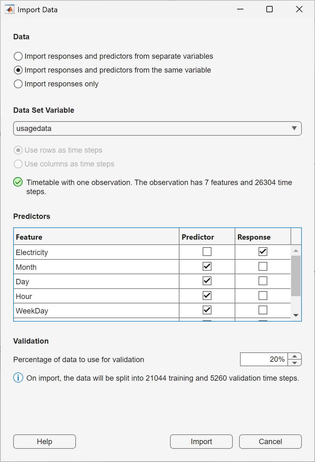
To import the predictors and responses into the app, click the New button on the toolstrip. The Import Data dialog box opens.

In the Import Data dialog box, select Import responses and predictors from the same variable and import the usagedata variable. Select Response for the Electricity feature, and verify that Predictor is selected for all other features. To use the last 20% of the time series as validation data, keep the default value of 20% in the Percentage of data to use for validation box. Click Import.

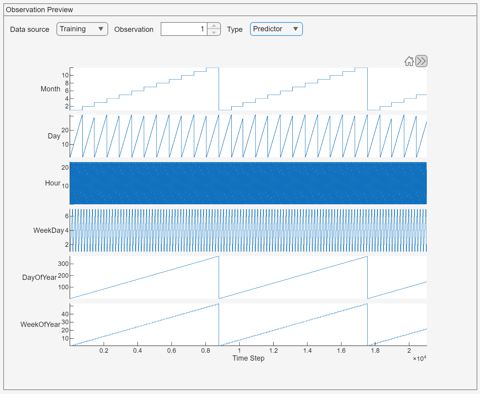
To check that you have imported the intended data, in the Data tab, view the Observation Preview pane. In the Observation Preview pane, set Type to Predictor to observe the periodicity of the temporal predictors.

Train Simple Nonautoregressive Multilayer Perceptron

Start with a simple, quick-to-train model: a small MLP. You can then try other models to improve accuracy.

On the toolstrip, in the Models gallery, click MLP (small). The Summary tab opens. Keep the default settings, and click Train on the toolstrip to train the model.

After training, assess the model performance. To view a plot of the model predictions on the validation set, under Plots, click Predict. This plot shows the model predictions on the validation set.

The model performs poorly on the latter part of the time series. To inspect the region of poor performance, use the Zoom button on the toolbar above the plot.

By default, deep learning models that you train in Time Series Modeler are not autoregressive and do not use previous values of the response variable. This approach works for many problems but fails to predict the later part of this series for this data set, where electricity consumption is higher than earlier values.

Train Autoregressive Multilayer Perceptron

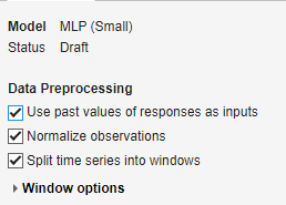
Create another small MLP model by clicking MLP (small). To create an autoregressive MLP with a lag of one time step, in the Summary tab, select Use past values of the responses as inputs. At time t, the model uses the predictor data at time t and the electricity consumption at time t-1. Click Train to train the model.

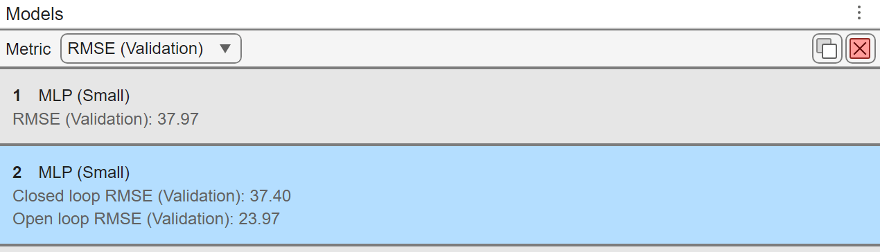
The training time of the autoregressive MLP is similar to that of the nonautoregressive MLP. For predictions, autoregressive models support two modes:

• Open-loop: Uses the actual response values as the autoregressive input. Use this prediction mode if you can access ground-truth data at prediction time. Prediction time is similar to that of a nonautoregressive MLP because the model processes the entire time series in a single pass.

• Closed-loop: Uses the predicted value of the model as the autoregressive input. Use this prediction mode if you cannot access ground-truth data at prediction time. Prediction time is slower compared to a nonautoregressive MLP because the model makes a forward pass at each time step to predict the next value using the output of previous predictions as inputs.

In this example, you likely have access to new data at prediction time, so use the open-loop mode. For example, use the measured value of electricity consumption at time t to predict the value at t+1.

The app reports the root mean squared error (RMSE) for both the closed-loop and open-loop modes. You can view these scores in the Models list at the left of the app. The open-loop RMSE is usually smaller because the ground-truth data continuously corrects the predictions of the model. In the closed-loop mode, errors in the predictions accumulate over time.

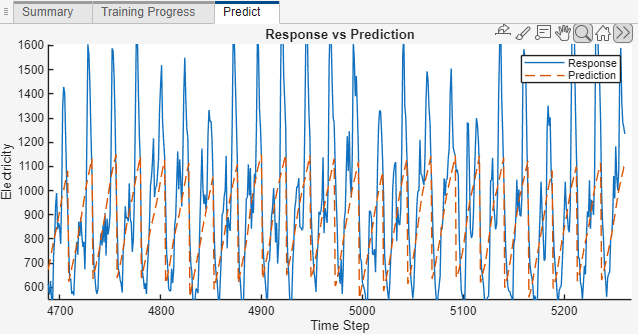
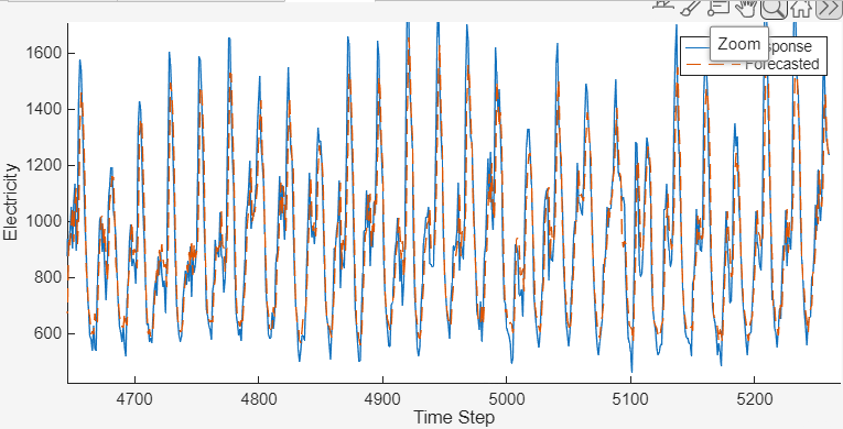
To assess the prediction performance of the model, click Predict. Generating the prediction plot takes some time because closed-loop prediction is computationally intensive.

Zoom in on time steps 4700 to 5300 by using the Zoom button in the top axes toolbar. Toggle the Prediction type dropdown between Closed loop and Open loop. Observe that open-loop prediction gives better results.

Train Neural Network with Longer Lag

The autoregressive MLP uses a lag of only one time step. To use longer lags, use a 1-D CNN. A 1-D CNN learns convolutional filters that span multiple time steps depending on the filter size.

Create a 1-D CNN by selecting Models > CNN (small). To make the model autoregressive, select Use past values of responses as inputs. Next, specify the model hyperparameters. Choosing model hyperparameters requires empirical analysis. For this example, use these settings:

• Network depth of two blocks.

• 16 filters per convolutional layer.

• Filter size of five. This setting corresponds to a maximum lag of five time steps.

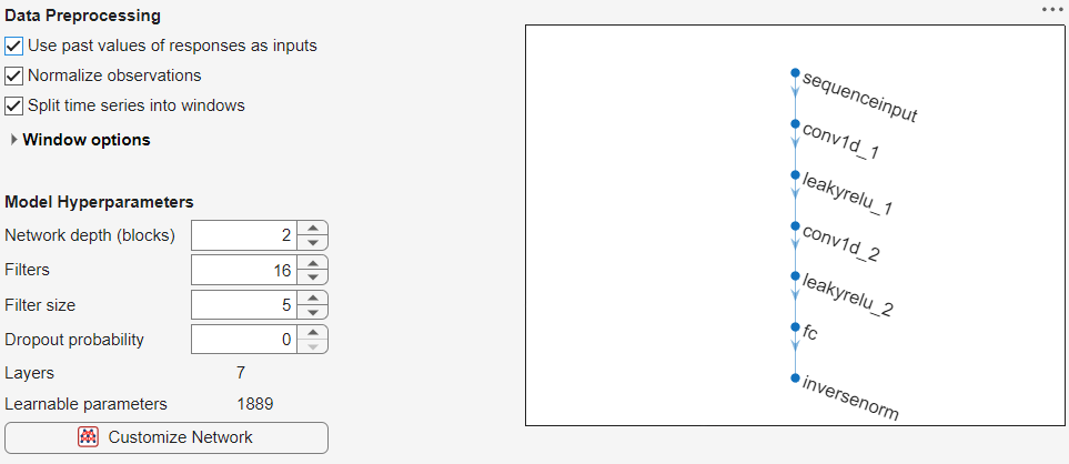
Click Train.

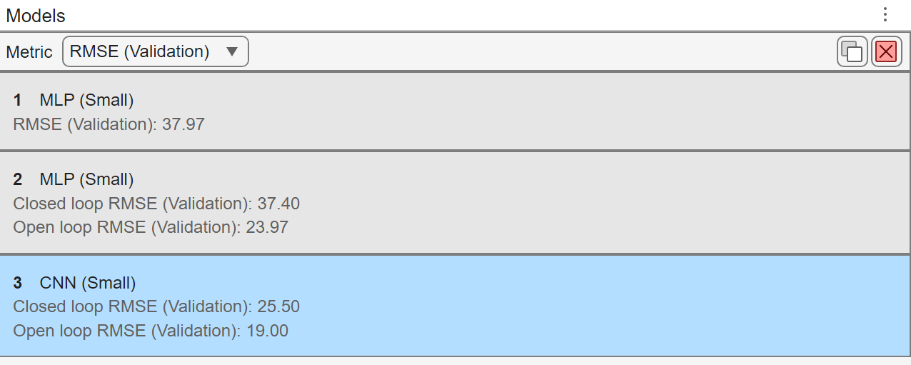
After training, observe that the open-loop RMSE of this model is smaller than those of the MLP models.

Generate MATLAB Code for Prediction

To make predictions with deep neural networks, especially autoregressive models, you must adjust many parameters. To support this workflow, you can use Time Series Modeler to generate MATLAB code for predicting on new data. You can then use this code to evaluate the trained network on a test set or gain more understanding of how autoregressive prediction works, or include the code in an extended data processing pipeline that contains a neural network. To generate MATLAB code for prediction for both the open- and close-loop modes on the toolstrip, select Export to Workspace and Generate Code.

References

[1] Dua, D. and Graff, C. (2019). UCI Machine Learning Repository [http://archive.ics.uci.edu/ml]. Irvine, CA: University of California, School of Information and Computer Science.