Build Custom Network for Time Series Modeling of a Virtual Sensor

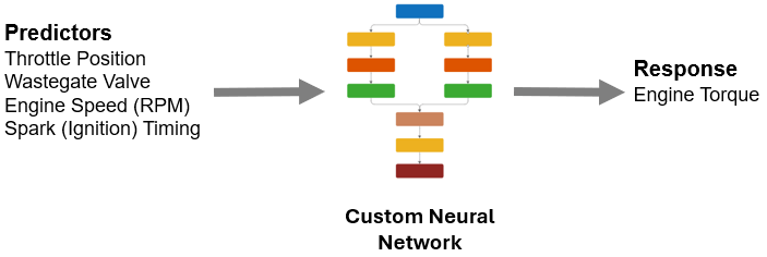
This example shows how to use the Time Series Modeler app to build and train a custom network for time series modeling of the nonlinear torque dynamics of a spark-ignition (SI) engine. In this example, you build a custom 1-D convolutional neural network with two branches.

Load Data

Load example engine data. In this example there is one response, engine torque. There are also four predictors: throttle position, wastegate valve area, engine speed, and spark timing. The data consists of a single time series with 29491 time steps.

For more information about this data set, see Neural State-Space Model of SI Engine Torque Dynamics (System Identification Toolbox).

load SIEngineData

Open the Time Series Modeler app.

timeSeriesModeler

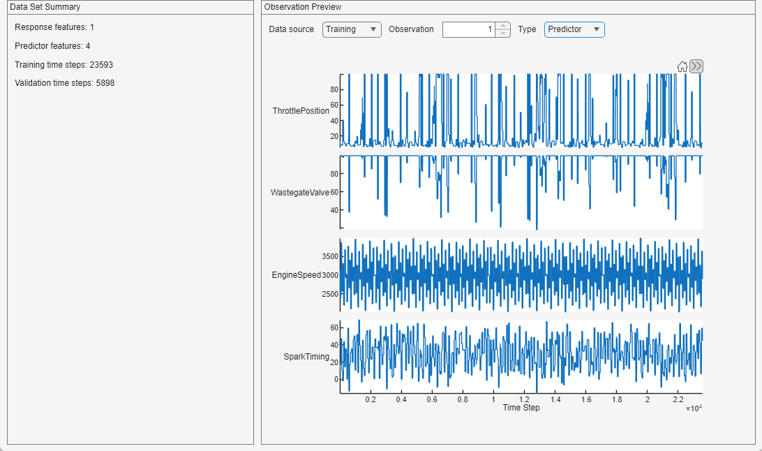
To import data, click New. In the Import Data dialog box, select Data to be Import responses and predictors from separate variables. Set responses to the responses workspace variable and the predictors to be the predictors workspace variable. Use 20% of the data for validation and 80% for training. Validation data is important for verifying the performance of your model on data that it does not see during training.

Click Import.

The app displays a summary of the data set and a preview of individual observations from the training and validation data, for both the responses and the predictors.

Build Model

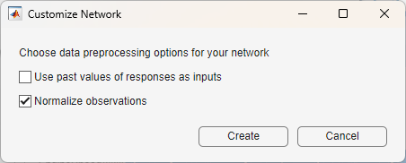
To create a custom model, in the Model gallery, select Blank Network. In the Customize Network dialog box, keep the default settings:

• To build a nonautoregressive model that does not use the responses as inputs, do not select Use past values of responses as inputs. A nonautoregressive model uses only the predictors as inputs.

• To normalize the observations, leave Normalize observations selected. Normalizing the predictors and responses can produce a better fit and prevent training from diverging.

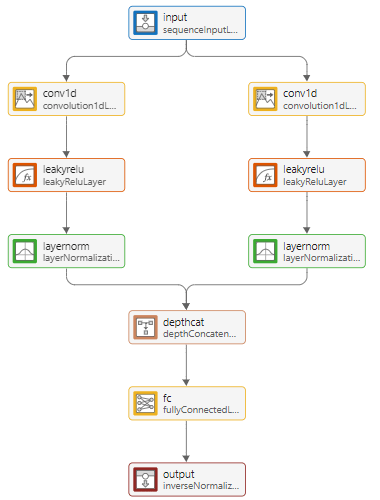
The Customize Network window opens. The app starts with an input layer and output layers on the Network canvas. Move the sequenceInputLayer to the top of the canvas and the fullyConnectedLayer and inverseNormalizationLayer to the bottom of the canvas. To build your network, add layers between the input and output layers.

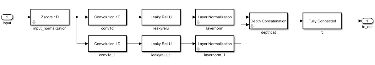
Build a convolutional neural network with two parallel branches. A convolutional neural network for time series data performs convolutions across time, learning filters that pick up features within a given number of time steps. Having two parallel branches allows each branch to learn filters that look at a different numbers of time steps.

To build your network, drag these layers from the Layer Library on to the canvas and connect them in order after the input layer.

1. convolution1dLayer with Padding set to causal. Causal padding ensures that the convolutional layers only incorporate information from past and present time steps, preventing data leakage from future values. If you do not use causal padding, then the model will appear to train well but perform poorly when you use it for predicting future values.

2. leakyReluLayer with Scale set to 0.3. This ensures the network can perform well with negative and positive values.

3. layerNormalizationLayer

Select the convolution1dLayer, leakyReluLayer, and layerNormalizationLayer layers and copy them. Connect the copied layers in the same way as the previous layers to create a second branch from the input layer. In the first convolution1dlayer, keep the default settings of FilterSize set to 3 and NumFilters set to 32. In the second 1-D convolutional layer, set FilterSize to 7 and NumFilters to 16. Using two branches with different filter sizes means the network can capture different feature representations.

Next, drag a depthConcatenationLayer onto the canvas and connect the output of the two layerNormalizationLayer layers to this layer. Finally, connect the output of the depthConcatenationLayer to the final fullyConnectedLayer.

For more information about how to build networks, see Build Networks with Deep Network Designer.

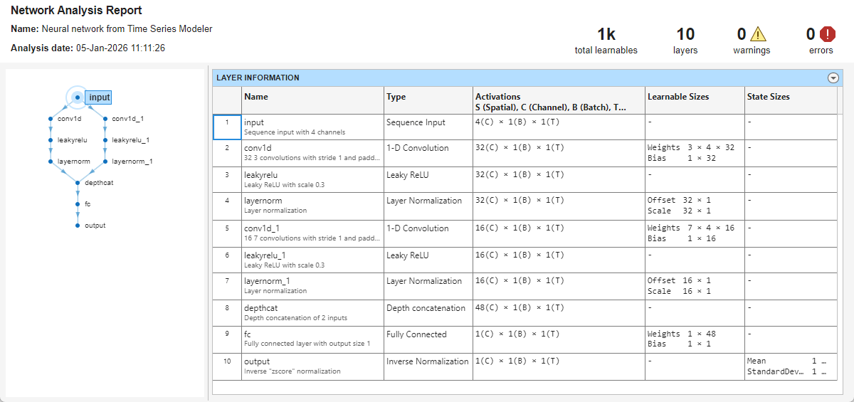
Once you have built your network, click Analyze to check that there are no warnings or errors.

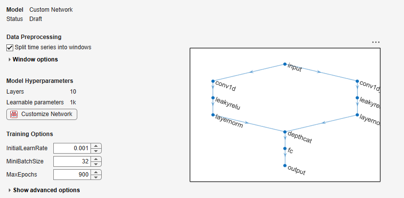
To accept the network architecture, click Accept Changes. The app displays a summary of the model, as well as data processing and training options. By default, the app splits the time series into multiple windows.

Set the MaxEpochs value to 900.

Train Model

To train the model, click Train. In the Axes toolbar above the plot, switch to the log scale to better see the change in the loss over the course of training.

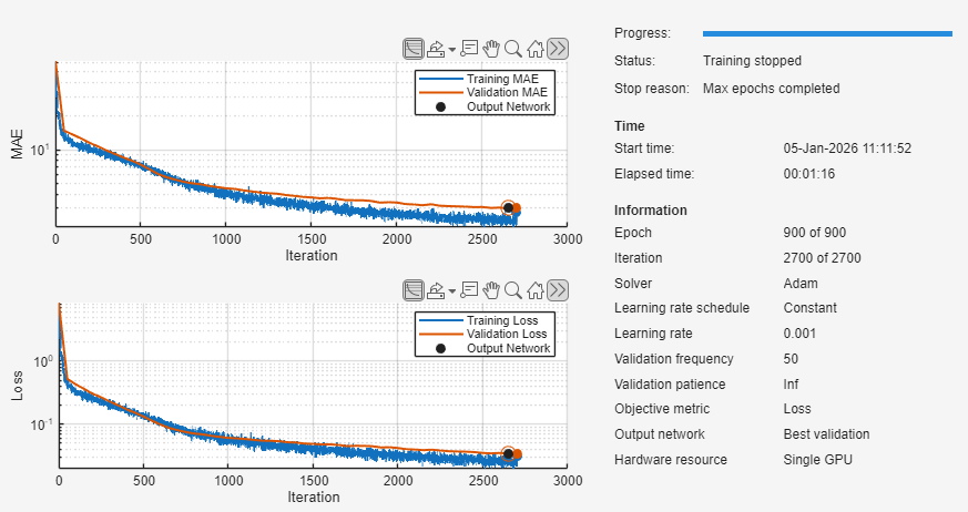
In this example, the model is overfitting slightly. To reduce the amount of overfitting, try adding a dropout layer. For more information, see Detect Overfitting When Training Model for Time Series Forecasting.

Assess Performance

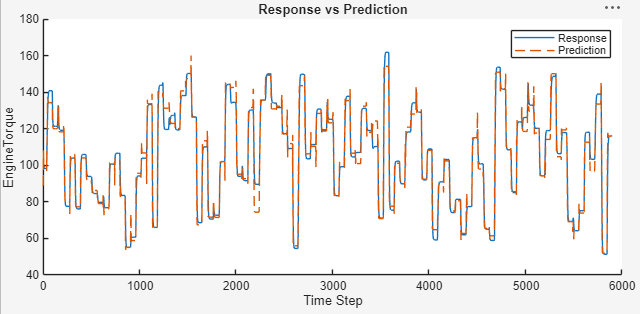
You can view the root mean squared error (RMSE) and mean absolute error (MAE) values for the trained model on the validation data in the Summary tab. To visualize how your model performs at predicting future values, in the Plots section, click Predict. The app displays the true time series values with the predicted values for comparison.

Export Model to Simulink and Generate C Code

Once you are happy with the trained model, click Export to Simulink. The app exports the model to layers blocks, with one block for each layer in the network.

To generate C code for the network, in the Simulink toolstrip, select Apps, then choose Simulink Coder. In the Simulink Coder tab, select Build > Generate Code.