Validate Simulation Results for Models with Internal Delays
This example shows the importance of validating the results of simulations with internal delays by varying sample time and comparing the continuous and discretized frequency responses.
Define the continuous time transfer function with an internal delay.
sys1 = tf([7174 5.514e+04 4.894e+04 991.2 7.848],...
   [1 296.2 4.455e+04 1.717e+05 171.3]);
sys2 = tf(1,[0.74 0 0],InputDelay=0.3);
sys = feedback(sys2*ss(sys1),1)
sys =

  A =
            x1       x2       x3       x4       x5       x6
   x1        0    -9695    -1011   -609.5   -73.42   -0.586
   x2        1        0        0        0        0        0
   x3        0    -2768   -296.2     -174   -20.96  -0.1673
   x4        0        0      256        0        0        0
   x5        0        0        0       32        0        0
   x6        0        0        0        0    0.125        0

  B =
         u1
   x1  7174
   x2     0
   x3  2048
   x4     0
   x5     0
   x6     0

  C =
          x1     x2     x3     x4     x5     x6
   y1      0  1.351      0      0      0      0

  D =
       u1
   y1   0

  (values computed with all internal delays set to zero)

  Internal delays (seconds): 0.3

Continuous-time state-space model.
Simulate the system in Simulink® using a stiff solver. Run the simulation for 100 seconds and log the output.
Tf = 100;
R= sim("checkSIM",ReturnWorkspaceOutputs="on");
tout = R.tout;
yout = R.yout;
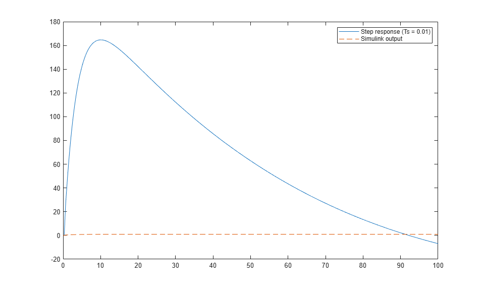
Compute the step response using a discrete time vector with Ts = 0.01. The response computed by step does not match the Simulink result. This mismatch indicates that the sample time is too large to capture the fast dynamics introduced by the internal delay.
t1 = 0:0.01:Tf;
y1 = step(sys,t1);
figure
plot(t1,y1,tout,yout,"--")
legend("Step response (Ts = 0.01)","Simulink output")
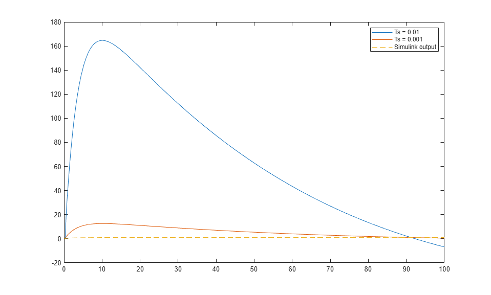
Reduce the sample time to Ts = 0.001. A smaller step size improves the agreement, but a noticeable gap remains.
t2 = 0:0.001:Tf;
y2 = step(sys,t2);
figure
plot(t1,y1,t2,y2,tout,yout,"--")
legend("Ts = 0.01","Ts = 0.001","Simulink output")
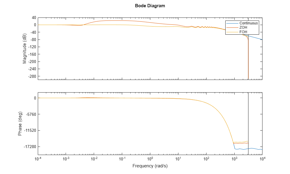
The accuracy of simulations with internal delays increases as the sample time decreases. To gauge whether the selected time step size is small enough, you can compare the frequency domain response of the continuous model with the model discretized with that sample time. Discretize the system using zero-order hold (ZOH) and first-order hold (FOH) with Ts = 0.001.
Ts = 0.001;
sysd_zoh = c2d(sys,Ts,"zoh");
sysd_foh = c2d(sys,Ts,"foh");
Warning: Discretization is only approximate due to internal delays. Use faster
sampling rate if discretization error is large.
Warning: Discretization is only approximate due to internal delays. Use faster
sampling rate if discretization error is large.
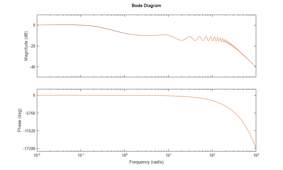
Compare the continuous system with discretized models in the frequency domain. The FOH discretization is in reasonable agreement but the ZOH discretization shows a large gap.
figure
bodeplot(sys,sysd_zoh,sysd_foh)
legend("Continuous","ZOH","FOH")
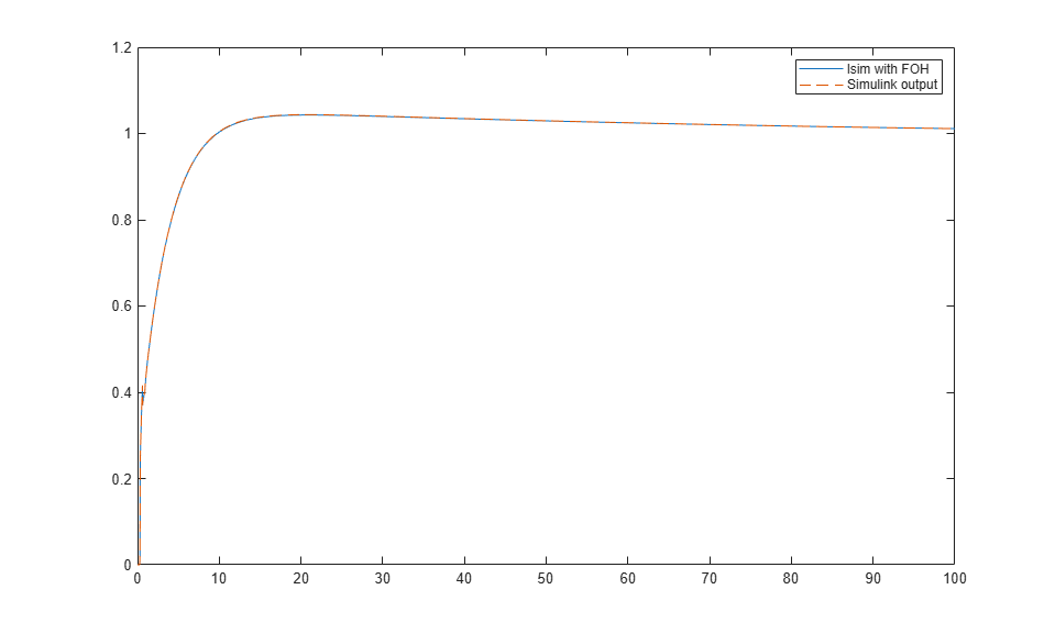
Compute the initial operating point and simulate the response using lsim with FOH. The result closely matches the Simulink output, confirming that FOH better represents the underlying continuous system.
t1 = 0:Ts:Tf;
u = ones(size(t1));
IC = findop(sys,u=0);
y1 = lsim(sys,u,t1,IC,"foh");

figure
plot(t1,y1,tout,yout,"--")
legend("lsim with FOH","Simulink output")
Repeat the simulation using ZOH with a very small step size. For ZOH, you have to reduce the step size drastically to erase the gap.
Ts = 1e-6;
t1 = 0:Ts:Tf;
y1 = step(sys,t1);

figure
plot(t1,y1,tout,yout,"--")
sysd_zoh2 = c2d(sys,Ts,"zoh");
Warning: Discretization is only approximate due to internal delays. Use faster
sampling rate if discretization error is large.
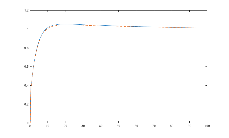
figure
bodeplot(sys,sysd_zoh2)
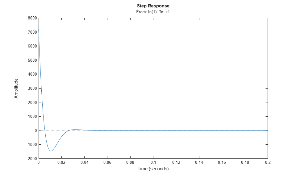
Examine the dynamics introduced by the internal delay. This atypical behavior is due to the extremely stiff (high frequency) response of the internal delay signal  (
( ) to the initial step. To analyze the contribution of internal delay signal, use the
 augdelay function.
asys = augdelay(sys);
stepplot(asys("delays",:),0.2)
See Also
augdelay | setDelayModel | c2d