Use Linearization Offsets to Help Compare Nonlinear and Linearized Responses
This example shows how to use offsets from linearization to facilitate the comparison of the nonlinear and linearized responses of a Simulink® model.
Airframe Model
This example uses the following Simulink model of the longitudinal dynamics of an airframe.
open_system('AirframeOL')
The goal is to compare the nonlinear and linearized pitch dynamics when changing the fin deflection delta by a small amount. This change is applied around a steady flight condition, for a steady climb with flight path angle gamma of 20 degrees. This comparison is done for several air speeds . Here, you start with .
To compute the corresponding operating condition, use operspec (Simulink Control Design) and findopOptions (Simulink Control Design) to trim fin deflection, thrust, and incidence according to the desired flight path.
Create an operating point specification object for the model using the model initial conditions.
V_t = 700;
gamma_t = 20;
opspec = operspec('AirframeOL');
Specify that the Position states are known and not at steady state. For the state values, specified in opspec.States(1).x, use the default values from the model initial condition.
opspec.States(1).Known = [1;1];
opspec.States(1).SteadyState = [0;0];
The third state specification includes the body axis angular rates u and w. Specify that both states are at steady state.
opspec.States(3).SteadyState = [1 1];
Specify that the second state, which corresponds to the angle of incidence Theta is at steady state, that is, pitch rate .
opspec.States(2).SteadyState = 1;
Set air speed V and flight path angle gamma as known and specify their values.
opspec.Outputs(2).Known = 1;
opspec.Outputs(2).y = V_t;
opspec.Outputs(5).Known = 1;
opspec.Outputs(5).y = gamma_t*pi/180;
Trim the model for the specified airspeed and flight path.
[op,report] = findop('AirframeOL',opspec);Operating point search report: ---------------------------------
opreport =
 Operating point search report for the Model AirframeOL.
 (Time-Varying Components Evaluated at time t=0)

Operating point search completed successfully using optimization.
States:
----------
    Min          x          Max        dxMin        dx         dxMax
___________ ___________ ___________ ___________ ___________ ___________

(1.) AirframeOL/Airframe Model/EOM/ Equations of Motion (Body Axes)/Position
     0           0           0         -Inf      657.7848       Inf
-3047.9999  -3047.9999  -3047.9999     -Inf      -239.4141      Inf
(2.) AirframeOL/Airframe Model/EOM/ Equations of Motion (Body Axes)/Theta
   -Inf       0.36591       Inf          0      -3.1183e-20      0
(3.) AirframeOL/Airframe Model/EOM/ Equations of Motion (Body Axes)/U,w
   -Inf      699.9007       Inf          0      -6.5008e-11      0
   -Inf       11.7886       Inf          0      -8.8732e-10      0
(4.) AirframeOL/Airframe Model/EOM/ Equations of Motion (Body Axes)/q
   -Inf     -3.1183e-20     Inf          0      -8.1784e-10      0

Inputs:
----------
   Min         u         Max
__________ __________ __________

(1.) AirframeOL/delta
   -Inf    -0.0070623    Inf
(2.) AirframeOL/thrust
   -Inf     3434.085     Inf

Outputs:
----------
    Min          y          Max
___________ ___________ ___________

(1.) AirframeOL/alpha
   -Inf      0.016842       Inf
(2.) AirframeOL/V
    700         700         700
(3.) AirframeOL/q
   -Inf     -3.1183e-20     Inf
(4.) AirframeOL/az
   -Inf       -9.1606       Inf
(5.) AirframeOL/gamma
  0.34907     0.34907     0.34907
Linearization of Airframe Pitch Dynamics
To linearize the model, first specify linearization input and output points.
io = [linio('AirframeOL/delta',1,'in');            % delta
      linio('AirframeOL/thrust',1,'in');           % Thrust
      linio('AirframeOL/Airframe Model',1,'out');  % alpha
      linio('AirframeOL/Airframe Model',2,'out');  % V
      linio('AirframeOL/Airframe Model',3,'out');  % q
      linio('AirframeOL/Airframe Model',5,'out')]; % gamma
Store linearization offset information in the info structure. Use the StoreOffsets option to return the linearization offsets along with the state-space matrices. These offsets capture the affine terms in the linearization about an operating condition .
linOpt = linearizeOptions('StoreOffsets',true);Use linearize to compute the linearized dynamics at the operating condition op computed in the previous section.
[G,~,info] = linearize('AirframeOL',op,io,linOpt);
G.u = {'delta','thrust'};
G.y = {'alpha','V','q','gamma'};
Attach the offsets to the linearized model G to take offsets into account in the time-domain simulations and enable direct comparison of the nonlinear and linearized responses.
G.Offsets = info.Offsets;
Verify that the derivative offset is close to zero since you linearized about a steady flight condition.
norm(G.Offsets.dx)
ans =
1.2085e-09
Nonlinear Simulation of Step Change
Use the AirframeSIM model to simulate the nonlinear response to a step change of a quarter degree in deflection delta.
open_system('AirframeSIM')
Here, that op.Inputs(1).u and op.Inputs(2).u are the trim input values and the step change has amplitude delta_step.
Initialize the simulation with the values computed by findop.
delta_step = 0.25;  % 1/4 deg step change
alpha_ini = report.Outputs(1).y;
q_ini = 0;
v_ini = V_t;
theta_ini = report.States(2).x;
Simulate and collect data.
t = 0:0.01:10;
sim('AirframeSIM',t)
Extract the signal data from simulation data.
delta = getElement(sigsOut,'delta');
delta = delta.Values.Data;
thrust = getElement(sigsOut,'thrust');
thrust = thrust.Values.Data;
alpha = getElement(sigsOut,'alpha');
alpha = alpha.Values.Data;
V = getElement(sigsOut,'V');
V = V.Values.Data;
q = getElement(sigsOut,'q');
q = q.Values.Data;
gamma = getElement(sigsOut,'gamma');
gamma = gamma.Values.Data;
Linear Simulation of Step Change
Use lsim to simulate the response of the linearized model G to the same input data. Set the initial condition to the offset, the steady-state condition you linearized about.
u = [delta,thrust*ones(numel(t),1)];
x_ini = G.offsets.x;  % initialize at trim
y = lsim(G,u,t,x_ini);
The nonlinear and linearized responses closely match for this air speed. Note how both responses are initially steady around the target values for , until the step change is applied at .
figure
tl = tiledlayout(2,2,'TileSpacing','Compact');
nexttile
plot(t,180/pi*alpha,t,180/pi*y(:,1),'r--')
title('alpha (deg)')
nexttile
plot(t,V,t,y(:,2),'r--')
title('V')
nexttile
plot(t,q,t,y(:,3),'r--')
title('q')
nexttile
plot(t,180/pi*gamma,t,180/pi*y(:,4),'r--')
title('gamma (deg)')
legend('nonlinear','linearized',Location="best")

Now, simulate without the offsets. This time the linearized response shows additional transients and biases, making the comparison less obvious.
G.Offsets = [];
yNoOff = lsim(G,u,t,x_ini);

figure
tiledlayout(2,2,'TileSpacing','Compact');
nexttile
plot(t,180/pi*alpha,t,180/pi*yNoOff(:,1),'r--')
title('alpha (deg)')
nexttile
plot(t,V,t,yNoOff(:,2),'r--')
title('V')
nexttile
plot(t,q,t,yNoOff(:,3),'r--')
title('q')
nexttile
plot(t,180/pi*gamma,t,180/pi*yNoOff(:,4),'r--')
title('gamma (deg)')
legend('nonlinear','linearized',Location="best")

Comparison for Different Air Speeds
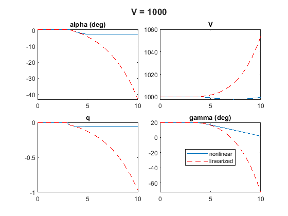
You can repeat this process for different air speeds , for example, and .


Results show the gap between nonlinear and linearized increases with air speed. For , the linearized response has an unstable mode which is not present in the nonlinear response. You can observe a similar deterioration when increasing the magnitude of the delta change.