Main Content

getrom

Obtain reduced-order models when using balanced truncation of normalized coprime factors method

Since R2023b

    Description

    Use getrom to obtain reduced-order models from a NCFBalancedTruncation model order reduction task created using reducespec. For the full workflow, see Task-Based Model Order Reduction Workflow.

    This method requires Robust Control Toolbox™ software.

    rsys = getrom(R,Name=Value) returns a reduced-order model rsys based on the options specified by name-value arguments.

    example

    [rsys,info] = getrom(R,___) also returns a structure info containing additional information, such as the left and right projector matrices.

    rsys = getrom(R) returns a simplified model rsys where all states associated with numerically zero Hankel singular values are removed. For this algorithm, the software simplifies the left normalized coprime factorization of the original model sys.

    getrom(R,'-help') returns help specific to the model order specification object R. The returned help shows the name-value arguments and syntaxes applicable to R.

    Examples

    collapse all

    This example shows how to obtain a reduced-order model using the balanced truncation of normalized coprime factors method.

    Load a 30-state plant model G.

    load ncfModel.mat G
    size(G)
    State-space model with 2 outputs, 3 inputs, and 30 states.
    

    Create a model order reduction task.

    R = reducespec(G,"ncf");

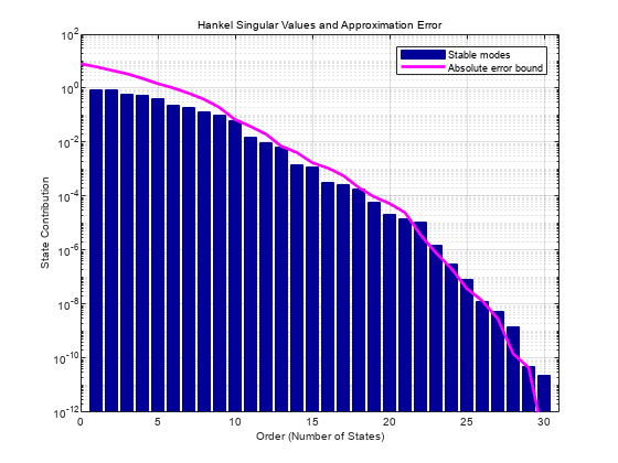
    To help you select a suitable target reduction order, examine the plot of Hankel singular values and approximation errors.

    Create the plot.

    view(R)

    MATLAB figure

    The function generates a Hankel singular value plot, which shows the relative energy contributions of each state in the coprime factorization of G, arranged in decreasing order by energy. The plot also shows the upper bound on the error between the original and reduced-order models that you obtain by truncating the states at that point. Examine this plot to choose the target order. For instance, for a maximum error of 0.01, you can reduce the model to 13th order.

    Examine the singular values of G and of the difference between G and Gred.

    Gred = getrom(R,MaxError=0.01);
    sigma(G,G-Gred)
    legend("G","G-Gred")

    MATLAB figure

    ans = 
      Legend (G, G-Gred) with properties:
    
             String: {'G'  'G-Gred'}
           Location: 'northeast'
        Orientation: 'vertical'
           FontSize: 9
           Position: [0.7184 0.7968 0.1675 0.0789]
              Units: 'normalized'
    
      Use GET to show all properties


    The difference is small across all frequencies, showing that the reduced-order model is a good approximation of the full-order model.

    This example show how to reduce controller order while preserving stability and robustness. This example requires Robust Control Toolbox™ software.

    When you use normalized coprime factorization (NCF) balanced truncation with getrom to reduce a plant G or controller K for which the closed-loop response feedback(G*K,eye(n)) is stable, the resulting closed-loop response is also stable as long as the approximation error of the reduced model does not exceed the robustness margin computed by ncfmargin. To see this benefit of NCF balanced truncation, load a plant G and design a controller for it. For this example, use ncfsyn (Robust Control Toolbox) to design the controller.

    load ncfStability.mat G
    size(G)
    State-space model with 1 outputs, 1 inputs, and 3 states.
    
    % shaping weights
    s = tf('s');
    W1 = 3.35*tf([1 20.89],[1 0]);
    W2 = 1;
    % controller
    [K,~,~,Kinfo] = ncfsyn(G,W1,W2); 
    size(K)
    State-space model with 1 outputs, 1 inputs, and 5 states.
    

    ncfsyn designs a controller by optimizing the ncfmargin robustness margin using a plant shaped by weighting functions W1 and W2 (see ncfsyn (Robust Control Toolbox)). To analyze margins with ncfmargin and reduce controller order, work with the shaped plant Gs and the controller Ks designed for it.

    Gs = Kinfo.Gs;
    Ks = Kinfo.Ks;

    Use ncfmargin (Robust Control Toolbox) to find the robustness margin of the system with the full-order controller. ncfsyn assumes a positive feedback loop while ncfmargin assumes negative feedback, so reverse the sign of the controller for this computation.

    emax = ncfmargin(Gs,-Ks)
    emax = 
    0.1956
    

    As long as the approximation error of the reduced-order controller does not exceed emax, stability of the closed-loop system is preserved.

    Create a model order reduction task using reducespec.

    R = reducespec(Ks,"ncf");
    R = process(R);

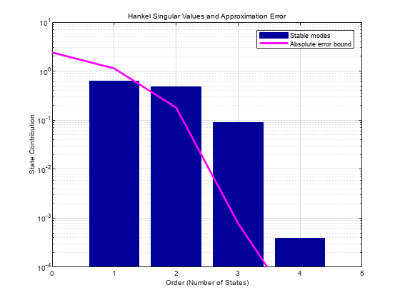
    To select the reduced order, visualize the errors associated with each target order.

    view(R)

    MATLAB figure

    Suppose that you can tolerate up to a 50% reduction in this margin in exchange for the computational benefit of a lower order controller.

    Obtain the reduced-order model such that the target error does not exceed emax/2.

    Ksr = getrom(R,MaxError=emax/2);
    size(Ksr)
    State-space model with 1 outputs, 1 inputs, and 3 states.
    

    The reduced-order controller yields a very similar stability margin to the original controller.

    ncfmargin(Gs,-Ksr)
    ans = 
    0.1949
    

    Reducing the controller order further leads to additional reduction in the stability margin. Reducing too far can lead to loss of closed-loop stability. For instance, try reducing to first order.

    Ksru = getrom(R,Order=1);
    ncfmargin(Gs,-Ksru)
    ans = 
    0
    

    Thus, for further analysis or implementation, use the third-order controller. To do so, convert Ksr, the reduced controller for Gs, into Kr, the reduced controller for G.

    Kr = W1*Ksr*W2;

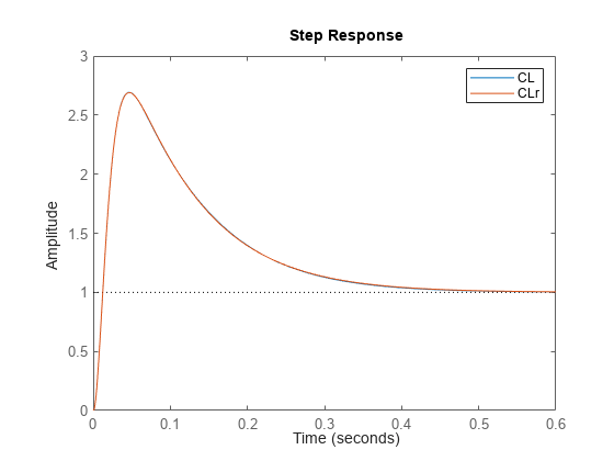
    To confirm that this controller is satisfactory, compare the closed-loop response to the response with the full-order controller. Again, reverse the sign of the controller to account for ncfsyn assuming positive feedback.

    CL = feedback(-G*K,1);
    CLr = feedback(-G*Kr,1);
    step(CL,CLr)
    legend

    MATLAB figure

    ans = 
      Legend (CL, CLr) with properties:
    
             String: {'CL'  'CLr'}
           Location: 'northeast'
        Orientation: 'vertical'
           FontSize: 9
           Position: [0.7596 0.7968 0.1264 0.0789]
              Units: 'normalized'
    
      Use GET to show all properties


    The large overshoot in this case is due to instability of the original plant G.
    Input Arguments

    collapse all

    Model order reduction specification object, specified as an NCFBalancedTruncation object created using reducespec.

    Name-Value Arguments

    Specify optional pairs of arguments as Name1=Value1,...,NameN=ValueN, where Name is the argument name and Value is the corresponding value. Name-value arguments must appear after other arguments, but the order of the pairs does not matter.

    Example: rsys = getrom(R,Order=[10,14])

    Desired order of the reduced-order model, specified as a nonnegative scalar or vector.

    • To obtain a single reduced-order model rsys, use a scalar.

    • To obtain an array of reduced models rsys, use a vector.

      For example, if you specify rsys = getrom(R,Order=[5,8,11]), rsys is a 3-by-1 model array containing reduced-order models with orders of 5, 8, and 11.

    The arguments Order, MaxError, and MinEnergy are mutually exclusive. You can specify only one of these arguments at a time.

    Maximum approximation error, specified as a nonnegative scalar or vector.

    • To obtain a single reduced-order model rsys, use a scalar.

    • To obtain an array of reduced models rsys, use a vector.

      For example, if you specify rsys = getrom(R,MaxError=[1e-3,1e-5,1e-7]), rsys is a 3-by-1 model array containing reduced-order models with the specified error bounds.

    The function selects the lowest order for which the error does not exceed the value you specify for this argument.

    The arguments Order, MaxError, and MinEnergy are mutually exclusive. You can specify only one of these arguments at a time.

    Minimum bound on the normalized energy, specified as a nonnegative scalar or vector.

    • To obtain a single reduced-order model rsys, use a scalar.

    • To obtain an array of reduced models rsys, use a vector.

      For example, if you specify rsys = getrom(R,MinEnergy=[1e-3,1e-5]), rsys is a 2-by-1 model array containing reduced-order models with the specified minimum normalized energies of the states.

    The function discards all the states that have normalized energies lower than the value you specify for this argument.

    The arguments Order, MaxError, and MinEnergy are mutually exclusive. You can specify only one of these arguments at a time.

    Output Arguments

    collapse all

    Reduced-order model, returned as a state-space model or an array of state-space models.

    Additional information about the reduced-order model, returned as a structure or structure array.

    • If rsys is a single state-space model, then info is a structure.

    • If rsys is an array of state-space models, then info is a structure array with the same dimensions as rsys.

    Each info structure has this field:

    FieldDescription
    RLNCF

    Left normalized coprime factorization of the reduced-order state-space model, returned as a state-state space model.

    If rsys has Ny outputs and Nu outputs, RLNCF has Ny outputs and Ny+Nu inputs.

    Version History

    Introduced in R2023b