Main Content

getrom

Obtain reduced-order models when using modal truncation method

Since R2023b

    Description

    Use getrom to obtain reduced-order models from a ModalTruncation or SparseModalTruncation model order reduction task. For the full workflow, see Task-Based Model Order Reduction Workflow.

    rsys = getrom(R,Name=Value) returns a reduced-order model rsys based on the options specified by one or more name-value arguments.

    example

    [rsys,info] = getrom(R,___) also returns a structure info containing additional information, such as the left and right projector matrices.

    example

    rsys = getrom(R) returns a modal decomposition of the original model sys.

    • For the ordinary modal truncation, this syntax returns:

      • The modal form (same as modalreal) of sys when R.Options.ModeOnly is set to false

      • The Schur form when R.Options.ModeOnly is set to true.

    • For sparse modal truncation, this syntax returns a reduced modal form based on the subset of modes computed by the algorithm. This subset is controlled by the R.Options.Focus or R.Options.MaxOrder options

    getrom(R,'-help') returns help specific to the model order specification object R. The returned help shows the name-value arguments and syntaxes applicable to R.

    Examples

    collapse all

    This example shows how to obtain a reduced-order model for a linear time-invariant (LTI) model using the modal truncation method. In this example, you reduce a high-order model with a focus on the dynamics in a particular frequency range and damping.

    Load a model and examine its frequency response.

    load('highOrderModel.mat','G')
    bodeplot(G)

    MATLAB figure

    G is a 48th-order model with several large peak regions around 5.2 rad/s, 13.5 rad/s, and 24.5 rad/s, and smaller peaks scattered across many frequencies.

    Create a model order reduction task.

    R = reducespec(G,"modal");
    figure
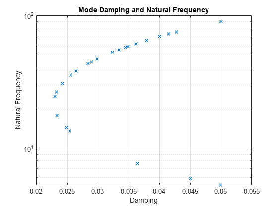
    view(R,"damp")

    Figure contains an axes object. The axes object with title Mode Damping and Natural Frequency, xlabel Damping, ylabel Natural Frequency contains a line object which displays its values using only markers.

    Suppose that for your application you are only interested in the dynamics between 10 rad/s and 40 rad/s with damping less than 0.04. Focus the model reduction on the region of interest to obtain a good match with a low-order approximation.

    rsys = getrom(R,Frequency=[10,40],Damping=[0.022 0.04]);
    bp = bodeplot(G,rsys,"r--");
    bp.PhaseMatchingEnabled = "on";
    legend("Full order","Reduced order");

    MATLAB figure

    The reduced-order model provides a good approximation for the specified targets.

    This example shows how to obtain a reduced-order model of a structural beam using the modal truncation method. For this example, consider a SISO sparse state-space model of a cantilever beam. This example uses the linearized model from the Linear Analysis of Cantilever Beam example.

    Load the beam model.

    load linBeam.mat
    size(sys)
    Sparse second-order model with 1 outputs, 1 inputs, and 3303 degrees of freedom.
    

    Plot the Bode response.

    bode(sys,w)

    MATLAB figure

    Create a model order reduction task.

    R = reducespec(sys,"modal");

    Set the Focus option to compute the eigenvalues only in the specified frequency range.

    R.Options.Focus = [0 5e5];

    Analyze the model and compute the derived information.

    R = process(R);
    size(R.Mode)
    ans = 1×2
    
        26     1


    The original model contains 26 modes. View the DC contribution of the modal components using the view function.

    view(R,"contrib")

    Figure contains an axes object. The axes object with title DC Contribution of Modal Components, xlabel Modal Component (Sorted), ylabel Normalized DC Contribution contains an object of type bar.

    Discard the modes with smaller contributions. For this example, discard all modes with DC contribution smaller than 1e-6. This results in a reduced model with 12 modes.

    [rsys,info] = getrom(R,MinDC=1e-6);

    Plot the bode responses.

    bode(sys,rsys,w)

    MATLAB figure

    The reduced-order model provides a good approximation for the original sparse model.

    Input Arguments

    collapse all

    Model order reduction specification object created using reducespec, specified as a ModalTruncation or SparseModalTruncation object.

    Name-Value Arguments

    Specify optional pairs of arguments as Name1=Value1,...,NameN=ValueN, where Name is the argument name and Value is the corresponding value. Name-value arguments must appear after other arguments, but the order of the pairs does not matter.

    Example: rsys = getrom(R,Frequency=[1e-2,1e6],Method="matchDC")

    Selected modes for the reduced-order model, specified as a vector. You can select modes in one of the following ways.

    • A vector containing index values into R.Modes.

    • A logical vector with the same size as R.Modes.

    The function retains the modes selected by these vectors. For example, if Selection is [1 2 3], it retains the modes R.Modes([1 2 3],:).

    Frequency range of interest, specified as a vector of form [Fmin,Fmax]. The function discards all the modes outside this range.

    Damping range of interest, specified as a vector of form [ζmin,ζmax]. The function discards all the modes outside this range.

    Minimum DC contribution bound for the reduced-order model, specified as a nonnegative scalar. The function discards all the modes with normalized DC contributions smaller than this value.

    State elimination method, specified as "matchDC" or "truncate". This argument specifies how the function eliminates the states with weak contribution.

    • The "matchDC" method preserves the DC gain (steady-state value of step response) and tends to match the time response better.

    • The "truncate" method tends to match the frequency response better. Use this method when you want to control the relative error.

    For the modal decomposition G(s) = G1(s) + G2(s) + D, where:

    • G1(s) contains the retained modes.

    • G2(s) contains the discarded modes.

    • D is the feedthrough term.

    The "truncate" method returns Gr(s) = G1(s) + D, and "matchDC" returns Gr(s) = G1(s) + D + G2(0) so that Gr(0) = G(0).

    Output Arguments

    collapse all

    Reduced-order model, returned as a state-space (ss) model.

    Additional information about the reduced-order model, returned as a structure with these fields.

    FieldDescription
    PLLeft projector matrix, returned as a matrix with dimensions Nx-by-Nxr, where Nx is the number of states in the original full-size model and Nxr is the number of states in the reduced-order model.
    PRRight projector matrix, returned as a matrix with dimensions Nx-by-Nxr, where Nx is the number of states in the original full-size model and Nxr is the number of states in the reduced-order model.

    More About

    collapse all

    Spectral Projector Matrices

    For the model-order reduction algorithms (excluding NCF balanced truncation), the function also returns the left and right spectral projector matrices in the info argument. For both "truncate" and "matchDC" methods, the matrices Ar, Br, Cr, Dr, and Er of the reduced-order model are related to the matrices A, B, C, D, and E of the original model by:

    • For explicit state-space models

      Ar=PLTAPR,Br=PLTB,Cr=CPr,Er=PLTPR=I

    • For descriptor state-space models

      Ar=PLTAPR,Br=PLTB,Cr=CPr,Er=PLTEPR

    Version History

    Introduced in R2023b