Linear Analysis of Cantilever Beam
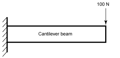
This example shows how to obtain a structural model of a beam and calculate the time and frequency response when it is subjected to an impulse force. For this example, consider a steel cantilever beam subject to a point load at the tip. Building the structural model requires Partial Differential Equation Toolbox™.
The steel beam is deformed by applying an external load of 100 N at the tip of the beam and then released. This example does not use any additional loading, so the displacement of the tip oscillates with an amplitude equal to the initial displacement from the applied force. This example follows the three-step workflow:
Construct a structural model of the beam.
Linearize the structural model to obtain a sparse linear model of the beam.
Analyze the time and frequency response of the linearized model.
Structural Model of Beam
Using Partial Differential Equation Toolbox, build a structural model and compute the impulse response. For an example of modeling a cantilever beam, see Dynamics of Damped Cantilever Beam (Partial Differential Equation Toolbox).
First construct the beam and specify the Young's modulus, Poisson's ratio, and mass density of steel. Specify the tip of the beam using the addVertex function.
gm = multicuboid(0.1,0.005,0.005);
E = 210E9;
nu = 0.3;
rho = 7800;
TipVertex = addVertex(gm,Coordinates=[0.05,0,0.005]);
Use createpde (Partial Differential Equation Toolbox) to construct the structural model and generate the mesh using the generateMesh (Partial Differential Equation Toolbox) command.
sModel = createpde(structural="transient-solid");
sModel.Geometry = gm;
msh = generateMesh(sModel);
Visualize the beam geometry using pdegplot (Partial Differential Equation Toolbox).
figure
pdegplot(sModel,FaceLabels="on");
title("Beam model")
![]()
Assign structural properties for the steel beam with the structuralProperties (Partial Differential Equation Toolbox) command and fix one end using structuralBC (Partial Differential Equation Toolbox).
structuralProperties(sModel,YoungsModulus=E,PoissonsRatio=nu,MassDensity=rho);
structuralBC(sModel,Face=5,Constraint="fixed");
You can calculate the vibration modes of the beam by solving the modal analysis model in a specified frequency range using solve (Partial Differential Equation Toolbox). For this beam, the first vibration mode is at 2639 rad/s as confirmed by the Bode plot in the Linear Analysis section of this example.
firstNF = 2639;
Tfundamental = 2*pi/firstNF;
To model an impulse (knock) on the tip of the beam, apply force for 2% of the fundamental period of oscillation (impulse) using structuralBoundaryLoad (Partial Differential Equation Toolbox). Specify the label force to use this force as a linearization input.
Te = 0.02*Tfundamental;
structuralBoundaryLoad(sModel,Vertex=TipVertex,Force=[0;0;-100], ...
                              EndTime=Te,Label="force");
Set initial conditions for the beam model using structuralIC (Partial Differential Equation Toolbox).
structuralIC(sModel,Velocity=[0;0;0]);
Compute the impulse response by solving the structural beam model.
ncycles = 10;
tsim = linspace(0,ncycles*Tfundamental,30*ncycles);
R1 = solve(sModel,tsim);
Visualize the oscillations at the tip of the beam.
figure
plot(tsim,R1.Displacement.uz(TipVertex,:))
title('Vertical Displacement of Beam Tip')
legend('Structural PDE model')
xlabel('Time')
ylabel('Displacement')
![]()
Structural Model Linearization
For this beam model, you want to obtain a linear model (transfer function) from the force applied at the tip to the z-displacement of the tip.
To do so, first specify the inputs and outputs of the linearized model in terms of the structural model. Here, the input is the force specified with structuralBoundaryLoad (Partial Differential Equation Toolbox) and the output is the z degree of freedom of the tip vertex.
linearizeInput(sModel,"force");
linearizeOutput(sModel,Vertex=TipVertex,Component="z");
Then, use the linearize (Partial Differential Equation Toolbox) command to extract the mechss model.
sys = linearize(sModel)
Sparse continuous-time second-order model with 1 outputs, 3 inputs, and 3303 degrees of freedom.
Model Properties

Use "spy" and "showStateInfo" to inspect model structure.
Type "help mechssOptions" for available solver options for this model.
The linearized model has three inputs corresponding to the x, y, and z components of the force applied to the tip vertex.
sys.InputName
ans = 3×1 cell array
    "'force_x'"
    "'force_y'"
    "'force_z'"
In the linearized model, select the z component of the force.
sys = sys(:,3)
Sparse continuous-time second-order model with 1 outputs, 1 inputs, and 3303 degrees of freedom.
Model Properties

Use "spy" and "showStateInfo" to inspect model structure.
Type "help mechssOptions" for available solver options for this model.
The resultant model is defined by the following set of equations:
Use spy to visualize the sparsity of the mechss model sys.
figure
spy(sys)
![]()
Linear Analysis
Choose 'tfbdf3' as the differential algebraic equation (DAE) solver.
sys.SolverOptions.DAESolver = "trbdf3";Use bode to compute the frequency response of the linearized model sys.
w = logspace(2,6,1000);
figure
bode(sys,w)
grid
title("Frequency Response from Force to Tip Vertical Displacement")![]()
The Bode plot shows that the first vibration mode is at approximately firstNF = 2639 rad/s.
Next use lsim to simulate the impulse response and compare with the results from the PDE model. To limit the error due to linear interpolation of the force between samples, use a step size of Te/5. Recall that the force is applied at the beam tip for the short time interval [0 Te].
h = Te/5;
t = 0:h:ncycles*Tfundamental;
u = zeros(size(t));
u(t<=Te) = -100;

y = lsim(sys,u,t);
figure
plot(t,y,tsim,R1.Displacement.uz(TipVertex,:))
title({'Comparison of Sparse LSIM Response';...
        'with PDE Model Simulation'})
legend("Linearized model','Structural PDE model")
xlabel("Time")
ylabel("Displacement")![]()
The linear response from lsim closely matches the transient simulation of the structural model obtained in the first step.
See Also
showStateInfo | spy | mechss | solve (Partial Differential Equation Toolbox) | structuralBC (Partial Differential Equation Toolbox) | structuralIC (Partial Differential Equation Toolbox) | createpde (Partial Differential Equation Toolbox) | linearize (Partial Differential Equation Toolbox) | linearizeInput (Partial Differential Equation Toolbox) | linearizeOutput (Partial Differential Equation Toolbox)