주요 콘텐츠

optimizePoseGraph

Optimize nodes in pose graph

Description

The optimizePoseGraph function optimizes the poses within a pose graph such that they comply with the edge constraints as much as possible.

This pose graph optimization assumes all edge constraints and loop closures are valid. To consider trimming edges based on bad loop closures, see the trimLoopClosures function.

Note

Computer Vision Toolbox™ is required if the pose graph is represented as a digraph object. Use the createPoseGraph object function of imageviewset (Computer Vision Toolbox) or pcviewset (Computer Vision Toolbox) to create the digraph object of the required format, where node estimates are represented by rigidtform3d and edge constraints are represented by either rigidtform3d or simtform3d. If digraph edge information matrix is not supplied, it is assumed to be identity by default.

This comparison chart shows the corresponding pose format for the different representations of pose graph:

Pose Graph RepresentationsPose Formats
poseGraph objectPoses are 3-element row vectors of the form [x, y, yaw].
poseGraph3D objectPoses are seven-element row vectors of the form[x, y, z, qw, qx, qy, qz]. Note the sequence in the quaternion part.
digraph objectPoses are rigidtform3d (Image Processing Toolbox) or simtform3d (Image Processing Toolbox) objects. This representation requires Computer Vision Toolbox.

updatedGraph = optimizePoseGraph(poseGraph) adjusts the poses based on their edge constraints defined in the specified graph to improve the overall graph. You optimize either a 2-D or 3-D pose graph. The returned pose graph has the same topology with updated nodes.

example

updatedGraph = optimizePoseGraph(poseGraph,solver) specifies the solver type for optimizing the pose graph.

[updatedGraph,solutionInfo] = optimizePoseGraph(___) returns additional statistics about the optimization process in solutionInfo using any of the previous syntaxes.

[___] = optimizePoseGraph(___,Name,Value) specifies additional options using one or more Name,Value pairs. For example, 'MaxIterations',1000 increases the maximum number of iterations to 1000.

Examples

collapse all

Optimize a pose graph based on the nodes and edge constraints. The pose graph used in this example is taken from the MIT Dataset and was generated using information extracted from a parking garage.

Load the pose graph from the MIT dataset. Inspect the poseGraph3D object to view the number of nodes and loop closures.

load parking-garage-posegraph.mat pg
disp(pg);
  poseGraph3D with properties:

               NumNodes: 1661
               NumEdges: 6275
    NumLoopClosureEdges: 4615
     LoopClosureEdgeIDs: [128 129 130 132 133 134 135 137 138 139 140 142 143 144 146 147 148 150 151 204 205 207 208 209 211 212 213 215 216 217 218 220 221 222 223 225 226 227 228 230 231 232 233 235 236 237 238 240 241 242 243 244 … ] (1×4615 double)
        LandmarkNodeIDs: [1×0 double]

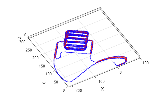
Plot the pose graph with IDs off. Red lines indicate loop closures identified in the dataset.

title('Original Pose Graph')
show(pg,'IDs','off');
view(-30,45)

Figure contains an axes object. The axes object with xlabel X, ylabel Y contains 3 objects of type line. One or more of the lines displays its values using only markers

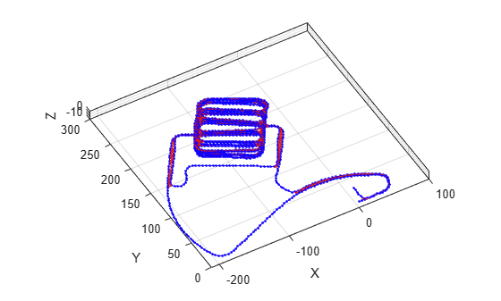
Optimize the pose graph. Nodes are adjusted based on the edge constraints and loop closures. Plot the optimized pose graph to see the adjustment of the nodes with loop closures.

updatedPG = optimizePoseGraph(pg);
figure
title('Updated Pose Graph')
show(updatedPG,'IDs','off');
view(-30,45)

Figure contains an axes object. The axes object with xlabel X, ylabel Y contains 3 objects of type line. One or more of the lines displays its values using only markers

Input Arguments

collapse all

2-D or 3-D pose graph, specified as a poseGraph, poseGraph3D, digraph object.

To use the digraph object, generate the pose graph using createPoseGraph from an imageviewset or pcviewset object. You must have Computer Vision Toolbox and the solver must be set to "g2o-levenberg-marquardt". The solver ignores the LoopClosuresToIgnore and FirstNodePose name-value arguments if specified.

The edges of digraph object are described by simtform3d (Image Processing Toolbox) or rigidtform3d (Image Processing Toolbox) objects.

Pose graph solver, specified as either "builtin-trust-region" or "g2o-levenberg-marquardt". To tune either solver, use the name-value arguments for that solver.

Note

If the pose graph is a digraph object, then the solver argument must be set to "g2o-levenberg-marquardt", and the solver ignores the LoopClosuresToIgnore and FirstNodePose name-value arguments during optimization if specified.

Name-Value Arguments

expand all

Specify optional pairs of arguments as Name1=Value1,...,NameN=ValueN, where Name is the argument name and Value is the corresponding value. Name-value arguments must appear after other arguments, but the order of the pairs does not matter.

Example: 'MaxTime', 300

Note

Depending on the solver input, the function supports different name-value arguments.

If the solver input is set to "builtin-trust-region":

expand all

Maximum time allowed, specified as the comma-separated pair consisting of 'MaxTime' and a positive numeric scalar in seconds. The optimizer exits after it exceeds this time.

Lower bound on the norm of the gradient, specified as the comma-separated pair consisting of 'GradientTolerance' and a scalar. The norm of the gradient is calculated based on the cost function of the optimization. If the norm falls below this value, the optimizer exits.

Lower bound on the change in the cost function, specified as the comma-separated pair consisting of 'FunctionTolerance' and a scalar. If the cost function change falls below this value between optimization steps, the optimizer exits.

Lower bound on the step size, specified as the comma-separated pair consisting of 'StepTolerance' and a scalar. If the norm of the optimization step falls below this value, the optimizer exits.

Initial trust region radius, specified as a scalar.

Display intermediate iteration information on the MATLAB® command line, specified as the comma-separated pair consisting of 'VerboseOutput' and either 'off' or 'on'.

IDs of loop closure edges in poseGraph, specified as the comma-separated pair consisting of 'LoopClosuresToIgnore' and a vector. To get edge IDs from the pose graph, use findEdgeID.

Pose of the first node in poseGraph, specified as the comma-separated pair consisting of 'FirstNodePose' and a pose vector.

For poseGraph (2-D), the pose is an [x y theta] vector, which defines the relative xy-position and orientation angle, theta.

For poseGraph3D, the pose is an [x y z qw qx qy qz] vector, which defines the relative xyz-position and quaternion orientation, [qw qx qy qz].

Note

Many other sources for 3-D pose graphs, including .g2o formats, specify the quaternion orientation in a different order, for example, [qx qy qz qw]. Check the source of your pose graph data before adding nodes to your poseGraph3D object.

If the solver input is set to "g2o-levenberg-marquardt":

expand all

Maximum number of iterations, specified as the comma-separated pair consisting of 'MaxIterations' and a positive integer. The optimizer exits after it exceeds this number of iterations.

Maximum time allowed, specified as the comma-separated pair consisting of 'MaxTime' and a positive numeric scalar in seconds. The optimizer exits after it exceeds this time.

Lower bound on the change in the cost function, specified as the comma-separated pair consisting of 'FunctionTolerance' and a scalar. If the cost function change falls below this value between optimization steps, the optimizer exits.

Display intermediate iteration information on the MATLAB command line, specified as the comma-separated pair consisting of 'VerboseOutput' and either 'off' or 'on'.

Output Arguments

collapse all

Optimized 2-D or 3-D pose graph, returned as a poseGraph or poseGraph3D object.

Statistics of optimization process, returned as a structure with these fields:

  • Iterations — Number of iterations used in optimization.

  • ResidualError — Value of cost function when optimizer exits.

  • Exit Flag — Exit condition for optimizer:

    • 1 — Local minimum found.

    • 2 — Maximum number of iterations reached. See MaxIterations name-value argument.

    • 3 — Algorithm timed out during operation.

    • 4 — Minimum step size. The step size is below the StepTolerance name-value argument.

    • 5 — The change in error is below the minimum.

    • 8 — Trust region radius is below the minimum set in InitialTrustRegionRadius.

References

[1] Grisetti, G., R. Kummerle, C. Stachniss, and W. Burgard. "A Tutorial on Graph-Based SLAM." IEEE Intelligent Transportation Systems Magazine. Vol. 2, No. 4, 2010, pp. 31–43. doi:10.1109/mits.2010.939925.

[2] Carlone, Luca, Roberto Tron, Kostas Daniilidis, and Frank Dellaert. "Initialization Techniques for 3D SLAM: a Survey on Rotation Estimation and its Use in Pose Graph Optimization." 2015 IEEE International Conference on Robotics and Automation (ICRA). 2015, pp. 4597–4604.

Extended Capabilities

expand all

Version History

Introduced in R2019b