Design of Decimators and Interpolators

This example shows how to design filters for decimation and interpolation of discrete sequences.

Role of Lowpass Filtering in Rate Conversion

Rate conversion is the process of changing the rate of a discrete signal to obtain a new discrete representation of the underlying continuous signal. The process involves uniform downsampling and upsampling. Uniform downsampling by a rate of N refers to taking every N-th sample of a sequence and discarding the remaining samples. Uniform upsampling by a factor of N refers to the padding of N-1 zeros between every two consecutive samples.

x = 1:3

x = 1×3

     1     2     3

L = 3; % upsampling rate
M = 2; % downsampling rate

% Upsample and downsample
xUp   = upsample(x,L)

xUp = 1×9

     1     0     0     2     0     0     3     0     0

xDown = downsample(x,M)

xDown = 1×2

     1     3

Both these basic operations introduce signal artifacts. Downsampling introduces aliasing, and upsampling introduces imaging. To mitigate these effects, use a lowpass filter.

• When downsampling by a rate of $$N$$, apply a lowpass filter prior to downsampling to limit the input bandwidth, and thus eliminate spectrum aliasing. This is similar to an analog lowpass filter (LPF) used in Analog/Digital (A/D) converters. Ideally, such an antialiasing filter has a unit gain and a cutoff frequency of $${\omega }_c=\frac{1}{N}{\omega }_N$$, here $${\omega }_N$$ is the Nyquist frequency of the signal. For the purposes of this example, assume normalized frequencies (i.e. $${\omega }_N=1$$) throughout the discussion, so the underlying sampling frequency is insignificant.

• When upsampling by a rate of $$N$$, apply a lowpass filter after upsampling, this filter is known as an anti-imaging filter. The filter removes the spectral images of the low-rate signal. Ideally, the cutoff frequency of this anti-imaging filter is $${\omega }_c=\frac{1}{N}$$ (like its antialiasing counterpart), while its gain is $$N$$.

Both upsampling and downsampling operations of rate $$N$$ require a lowpass filter with a normalized cutoff frequency of $$\frac{1}{N}$$. The only difference is in the required gain and the placement of the filter (before or after rate conversion).

The combination of upsampling a signal by a factor of $$L$$, followed by filtering, and then downsampling by a factor of $$M$$ converts the sequence sample rate by a rational factor of $$\frac{L}{M}$$. You cannot commute the order of the rate conversion operation. A single filter that combines antialiasing and anti-imaging is placed between the upsampling and the downsampling stages. This filter is a lowpass filter with the normalized cutoff frequency of $${\omega }_c=\min (1/L,1/M)$$ and a gain of $$L$$.

While any lowpass FIR design function (e.g. fir1, firpm, or fdesign) can design an appropriate antialiasing and anti-imaging filter, the function designMultirateFIR is more convenient and has a simplified interface. The next few sections show how to use these functions to design the filter and demonstrate why designMultirateFIR is the preferred option.

Filtered Rate Conversion: Decimators, Interpolators, and Rational Rate Converters

Filtered rate conversion includes decimators, interpolators, and rational rate converters, all of which are cascades of rate change blocks with filters in various configurations.

Filtered Rate Conversion Using filter, upsample, and downsample Functions

Decimation refers to linear time-invariant (LTI) filtering followed by uniform downsampling. You can implement an FIR decimator using the following steps.

1. Design an antialiasing lowpass filter h.

2. Filter the input though h.

3. Downsample the filtered sequence by a factor of M.

% Define an input sequence
x = rand(60,1);

% Implement an FIR decimator
h = fir1(L*12*2,1/M); % an arbitrary filter
xDecim = downsample(filter(h,1,x), M);

Interpolation refers to upsampling followed by filtering. Its implementation is very similar to decimation.

xInterp = filter(h,1,upsample(x,L));

Lastly, rational rate conversion comprises of an interpolator followed by a decimator (in that specific order).

xRC = downsample(filter(h,1,upsample(x,L) ), M);

Filtered Rate Conversion Using System Objects

For streaming data, the System objects dsp.FIRInterpolator, dsp.FIRDecimator, and dsp.FIRRateConverter combine the rate change and filtering in a single object. For example, you can construct an interpolator as follows.

firInterp = dsp.FIRInterpolator(L,h);

Then, feed a sequence to the newly created object by a step call. Make sure that the time domain of your data runs along its columns, as these DSP System objects filters process along columns.

xInterp = firInterp(x);

Similarly, design and use decimators and rate converters.

firDecim = dsp.FIRDecimator(M,h); % Construct
xDecim = firDecim(x); % Decimate (step call)

firRC = dsp.FIRRateConverter(L,M,h); % Construct
xRC = firRC(x); % Convert sample rate (step call)

Using System objects is generally preferred, because System objects:

• Allow for a cleaner syntax.

• Keep a state, which you can use as initial conditions for the filter in subsequent step calls.

• Utilize a very efficient polyphase algorithm.

To create these objects, you need to specify the rate conversion factor and optionally the FIR coefficients. The next section shows how to design appropriate FIR coefficients for a given rate conversion filter.

Design a Rate Conversion Filter Using designMultirateFIR

The function designMultirateFIR(InterpolationFactor=L,DecimationFactor=M) automatically finds the appropriate scaling and cutoff frequency for a given rate conversion ratio $$L/M$$. When either of the InterpolationFactor or DecimationFactor arguments are omitted from the function call, they assume the value 1. Use the FIR coefficients returned by designMultirateFIR with dsp.FIRDecimator if InterpolationFactor=1, dsp.FIRInterpolator if DecimationFactor=1, or dsp.FIRRateConverter otherwise.

Design an interpolation filter:

L = 3;
bInterp = designMultirateFIR(InterpolationFactor=L); % Pure upsampling filter
firInterp = dsp.FIRInterpolator(L,bInterp);

Then, apply the interpolator to a sequence.

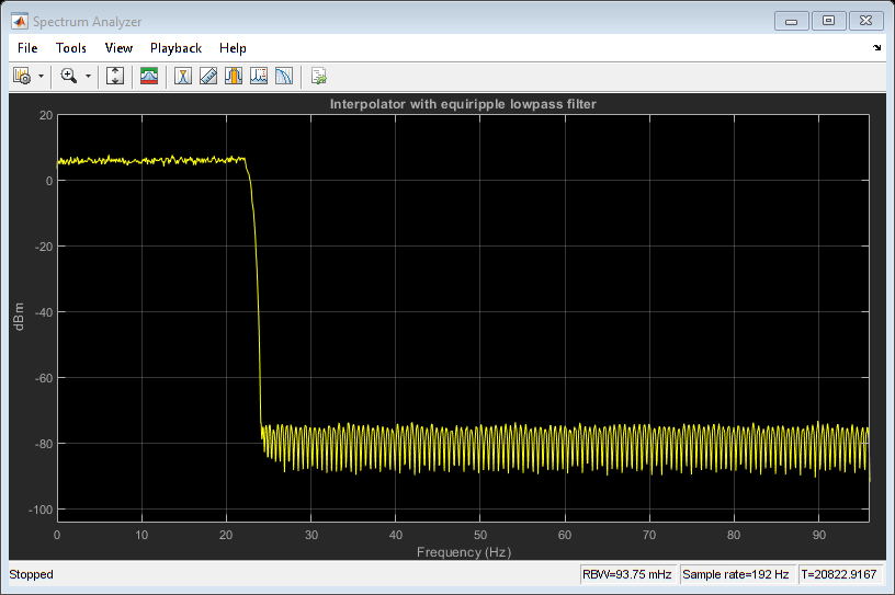
% Create a sequence
n = (0:89)';
f = @(t) cos(0.1*2*pi*t).*exp(-0.01*(t-25).^2)+0.2;
x = f(n);

% Apply interpolator
xUp = firInterp(x);
release(firInterp);

Examine the raw output of the interpolator and compare it to the original sequence.

plot_raw_sequences(x,xUp);

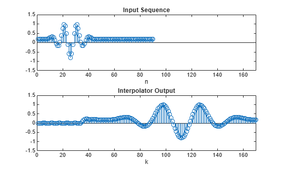
While there is some resemblance between the input x and the output xUp, there are several key differences. In the interpolated signal:

• The time domain is stretched (as expected).

• The signal has a delay, $$i_0$$, of half the length of the FIR length(h)/2.

• There is a transient response at the beginning.

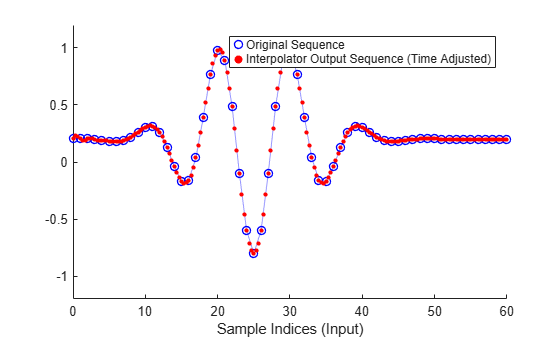
To compare, align and scale the time domains of the two sequences. An interpolated sample xUp[k] corresponds to an input time $$t[k]=\frac{1}{L}(k-i_0)$$.

nUp = (0:length(xUp)-1);
i0 = length(bInterp)/2;
plot_scaled_sequences(n,x,(1/L)*(nUp-i0),xUp,["Original Sequence",...
            "Interpolator Output Sequence (Time Adjusted)"],[0,60]);

Generally, if the input has a sample rate of $$FsIn$$, an input sample at time $$\frac{k}{F{s}_{in}}$$ it mapped to an output at time $$\frac{k}{F{s}_{out}}+D$$, here $$F{s}_{out}$$ is the output sample rate, and $$D$$ is a delay constant. When you use System objects, you can obtain the output delay and output rate using the outputDelay function.

[D,FsOut] = outputDelay(firInterp, FsIn = 1);
plot_scaled_sequences(n,x,nUp/FsOut-D,xUp,["Original Sequence",...
            "Interpolator Output Sequence (Time Adjusted)"],[0,60]);

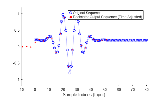
The same idea works for downsampling, where the time conversion for the output is $$t[k]=Mk-i_0$$.

M = 3;
bDecim = designMultirateFIR(DecimationFactor=M); % Pure downsampling filter
firDecim = dsp.FIRDecimator(M,bDecim);
xDown = firDecim(x);

Plot the original and time-adjusted sequence on the same scale and adjust for delay. They overlap perfectly.

nDown = (0:length(xDown)-1);
[D,FsOut] = outputDelay(firDecim);

plot_scaled_sequences(n,x,nDown/FsOut-D,xDown,["Original Sequence",...
            "Decimator Output Sequence (Time Adjusted)"],[-10,80]);

You can verify that indeed the returned FsOut and D have the expected values:

isequal(FsOut,1/M)

ans = logical
   1

isequal(D,length(bDecim)/2)

ans = logical
   1

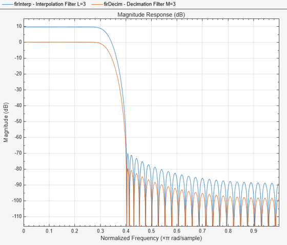
Visualize the magnitude responses of the upsampling and downsampling filters using filterAnalyzer. The two FIR filters are identical up to a different gain.

FA = filterAnalyzer(firInterp,firDecim); % Notice the gains in the passband
setLegendStrings(FA,["Interpolation Filter L="+num2str(L), ...
            "Decimation Filter M="+num2str(M)]);

You can treat general rational conversions the same way as upsampling and downsampling operations. The cutoff is $${\omega }_c=\min (\frac{1}{L},\frac{1}{M})$$ and the gain is $$L$$. The function designMultirateFIR figures that out automatically.

L = 5;
M = 2;
b = designMultirateFIR(InterpolationFactor=L,DecimationFactor=M);
firRC = dsp.FIRRateConverter(L,M,b);

Using rate conversion System objects in the automatic mode calls the designMultirateFIR internally.

firRC = dsp.FIRRateConverter(L,M,'auto');

Alternatively, a call to the designMultirateFIR function with the SystemObject flag set to true returns the appropriate System object.

firRC = designMultirateFIR(InterpolationFactor=L,DecimationFactor=M,SystemObject=true);

Compare the combined filter with the separate interpolation/decimation components.

firDecim  = dsp.FIRDecimator(M,'auto');
firInterp = dsp.FIRInterpolator(L,'auto');

FA = filterAnalyzer(firInterp,firDecim, firRC); % Notice the gains in the passband
setLegendStrings(FA,["Interpolation Filter L="+num2str(L),...
    "Decimation Filter M="+num2str(M), ...
    "Rate Conversion Filter L/M="+num2str(L)+"/"+num2str(M)]);

Once you create the FIRRateConverter object, perform rate conversion by a step call.

xRC = firRC(x);

Plot the filter input and output with the time adjustment given by $t[k] = \frac{1}{L}(Mk-i_0) = \frac{k}{Fs_{out}} -D $. As before, you can obtain the values of |FsOut| and |D| using |outputDelay|

[D,FsOut] = outputDelay(firRC);

Verify the frequency and delay values are as expected:

isequal(D, length(firRC.Numerator)/(2*L))

ans = logical
   1

isequal(FsOut, L/M)

ans = logical
   1

nRC = (0:length(xRC)-1)';

plot_scaled_sequences(n,x,nRC/FsOut-D,xRC,["Original Sequence",...
        "Rate Converter Output Sequence (time adjusted)"],[0,80]);

Design Rate Conversion Filters by Frequency Specification

You can design a rate conversion filter by specifying the input sample rate and output sample rate rather than the conversion ratio L:M. To do that, use the designRateConverter function, which offers a higher-level interface for designing rate conversion filters. You can specify absolute frequencies and designRateConverter deduces the conversion ratio, or you can specify the conversion ratio directly. For example, design a rate converter from 5 MHz to 8 MHz for an input signal with content up to 1 MHz (i.e. an input bandwidth of 40%).

src = designRateConverter(InputSampleRate=5e6, OutputSampleRate=8e6,...
            Bandwidth = 1e6, Verbose=true)

designRateConverter(InputSampleRate=5000000, OutputSampleRate=8000000, Bandwidth=1000000, StopbandAttenuation=80, MaxStages=Inf, CostMethod="estimate", Tolerance=0, ToleranceUnits="absolute")

Conversion ratio: 8:5
Input sample rate: 5e+06
Output sample rate: 8e+06

src = 
  dsp.FIRRateConverter with properties:

   Main
    InterpolationFactor: 8
       DecimationFactor: 5
        NumeratorSource: 'Property'
              Numerator: [1.4154e-04 1.6697e-04 0 -4.9375e-04 -0.0014 -0.0027 -0.0041 -0.0052 -0.0053 -0.0038 0 0.0063 0.0146 0.0237 0.0316 0.0357 0.0331 0.0216 0 -0.0307 -0.0672 -0.1038 -0.1325 -0.1442 -0.1302 -0.0834 0 0.1190 0.2675 … ] (1×69 double)

  Show all properties

In some cases, the resulting filter is a multistage cascade of FIR rate conversion filters. For example, resample an input sampled at 5 MHz to an output at a rate of 7 kHz. This rate converter is a cascade of 4 stages.

srccascade = designRateConverter(InputSampleRate=5e6,OutputSampleRate=7e3,...
                                Bandwidth = 2e3,Verbose=true)

designRateConverter(InputSampleRate=5000000, OutputSampleRate=7000, Bandwidth=2000, StopbandAttenuation=80, MaxStages=Inf, CostMethod="estimate", Tolerance=0, ToleranceUnits="absolute")

Conversion ratio: 7:5000
Input sample rate: 5e+06
Output sample rate: 7000

srccascade = 
  dsp.FilterCascade with properties:

         Stage1: [1×1 dsp.FIRDecimator]
         Stage2: [1×1 dsp.FIRDecimator]
         Stage3: [1×1 dsp.FIRDecimator]
         Stage4: [1×1 dsp.FIRRateConverter]
    CloneStages: true

For more information about cascaded rate converters see Multistage Rate Conversion.

Adjusting Lowpass FIR Design Parameters

The designMultirateFIR function allows you to adjust the FIR length, transition width, and stopband attenuation.

Adjust FIR Length

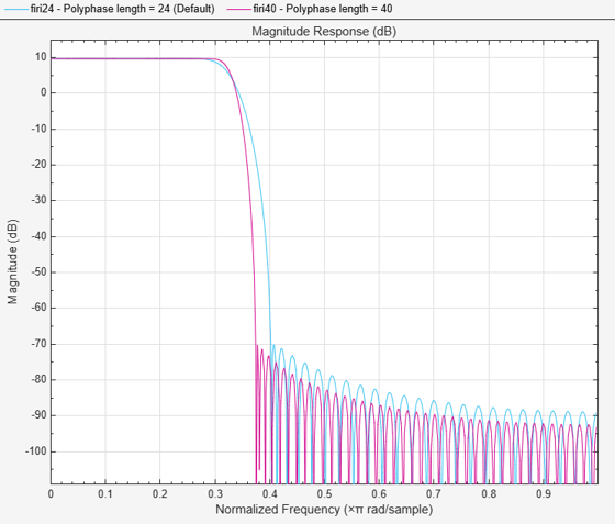
You can control the total FIR length through the InterpolationFactor and DecimationFactor the arguments, as well as the PolyphaseLength argument. The latter controls the length of each phase component, and has the default value of 24 samples (For more information, see Output Arguments). Design two such filters with different polyphase lengths.

% Unspecified PolyphaseLength defaults to 24
firi24 = designMultirateFIR(InterpolationFactor=3,SystemObject=true);

firi40 = designMultirateFIR(InterpolationFactor=3,...
                        PolyphaseLength=40,...
                        SystemObject=true);

Generally, a larger half-polyphase length yields steeper transitions. Visualize the two filters in filterAnalyzer.

FA = filterAnalyzer(firi24,firi40);
setLegendStrings(FA, ["Polyphase length = 24 (Default)","Polyphase length = 40"]);

Adjust Transition Width

Design the filter by specifying the desired transition width. The function derives the appropriate filter length automatically. Plot the resulting filter against the default design, and note the difference in the transition width.

TW = 0.02;
firiTW = designMultirateFIR(InterpolationFactor=3,...
                          TransitionWidth=TW,...
                          SystemObject=true);

FA = filterAnalyzer(firi24,firiTW);
setLegendStrings(FA,["Default Design (FIR Length = 72)",...
                    "Design with TW="+num2str(TW)+...
                    " (FIR Length="+num2str(length(firiTW))+")"]);

Special Case of Rate Conversion by 2: Halfband Interpolators and Decimators

A half-band lowpass filter ($${\omega }_c=\frac{1}{2}$$), can be used to perform sample rate conversion by a factor of 2. The dsp.FIRHalfbandInterpolator and dsp.FIRHalfbandDecimator objects are specialized System objects aimed at interpolation and decimation by a factor of 2 using halfband filters. These System objects are implemented using an efficient polyphase structure specific for that rate conversion, and work with normalized or absolute sample rates. Use the designHalfbandFIR function to design these objects.

There are two IIR counterparts dsp.IIRHalfbandInterpolator and dsp.IIRHalfbandDecimator, which can be even more efficient in some cases. Use the designHalfbandIIR function to design these objects.

Visualize the magnitude response using filterAnalyzer. In the case of interpolation, the filter retains most of the spectrum (between 0 to Fs/2 in absolute frequency units) while attenuating spectral images. For decimation, the filter passes about half of the band (between 0 to Fs/4 in absolute frequency units), and attenuates the other half in order to minimize aliasing. Set the amount of attenuation to any desired value using the StopbandAttenuation argument.

hbInterp = designHalfbandFIR(StopbandAttenuation = 80,TransitionWidth=0.1, ...
                            Structure='interp', SystemObject=true, Verbose=true)

designHalfbandFIR(TransitionWidth=0.1, StopbandAttenuation=80, DesignMethod="equiripple", Passband="lowpass", Structure="interp", PhaseConstraint="linear", Datatype="double", SystemObject=true)

hbInterp = 
  dsp.FIRHalfbandInterpolator with properties:

          Specification: 'Coefficients'
              Numerator: [-1.7896e-04 0 2.6955e-04 0 -4.6457e-04 0 7.4474e-04 0 -0.0011 0 0.0017 0 -0.0023 0 0.0032 0 -0.0044 0 0.0058 0 -0.0075 0 0.0097 0 -0.0123 0 0.0155 0 -0.0195 0 0.0243 0 -0.0304 0 0.0382 0 -0.0485 0 0.0628 0 … ] (1×95 double)
    FilterBankInputPort: false

  Show all properties

filterAnalyzer(hbInterp) % Notice gain of 2 (6 dB) in the passband

hbDecim  = designHalfbandFIR(StopbandAttenuation = 80,TransitionWidth=0.1, ...
                            Structure='decim', SystemObject=true, Verbose=true)

designHalfbandFIR(TransitionWidth=0.1, StopbandAttenuation=80, DesignMethod="equiripple", Passband="lowpass", Structure="decim", PhaseConstraint="linear", Datatype="double", SystemObject=true)

hbDecim = 
  dsp.FIRHalfbandDecimator with properties:

   Main
    Specification: 'Coefficients'
        Numerator: [-8.9482e-05 0 1.3477e-04 0 -2.3228e-04 0 3.7237e-04 0 -5.6658e-04 0 8.2825e-04 0 -0.0012 0 0.0016 0 -0.0022 0 0.0029 0 -0.0038 0 0.0048 0 -0.0062 0 0.0078 0 -0.0097 0 0.0122 0 -0.0152 0 0.0191 0 -0.0242 0 0.0314 0 … ] (1×95 double)

  Show all properties

filterAnalyzer(hbDecim)

Nyquist Filters: Interpolation Consistency v.s. Transition Overlap

A digital convolution filter $$h$$ is called an L-th Nyquist filter if it vanishes periodically every $$L$$ samples, except at the center index. In other words, sampling $$h$$ by a factor of $$L$$ yields an impulse:

$$h[kL]={\delta }_k$$

The $$L$$-th band ideal lowpass filter, $$h[m]=sinc(\frac{m}{L})$$, for example, is an $$L$$-th Nyquist filter. Another example of such a filter is a triangular window.

L=3;
t = linspace(-3*L,3*L,1024);
n = (-3*L:3*L);
hLP = @(t) sinc(t/L); 
hTri = @(t) (1-abs(t/L)).*(abs(t/L)<=1); 

plot_nyquist_filter(t,n,hLP,hTri,L);

The function designMultirateFIR uses the Kaiser-window design method by default, which naturally yields Nyquist designs obtained from weighted and truncated versions of ideal sinc filters (which are inherently Nyquist filters).

Nyquist filters are efficient to implement since an L-th fraction of the coefficients in these filters is zero, which reduces the number of required multiplication operations. This feature makes these filters efficient for both decimation and interpolation.

Interpolation Consistency

Nyquist filters retain the sample values of the input even after filtering. This behavior, which is called interpolation consistency, is not true in general, as shown here.

Interpolation consistency holds in Nyquist filters, since the coefficients equal zero every L samples (except at the center). The proof is straightforward. Assume that $$x_L$$ is the upsampled version of $$x$$ (with zeros inserted between samples) so that $$x_L[Ln]=x[n]$$, and that $$y=h*x_L$$ is the interpolated signal. Sample $$y$$ uniformly and get this equation.

$$y[nL]=(h*x_L)[Ln]=\sum _{k}h[Ln-k]x_L[k]=\sum _m\underset{\delta [L(n-m)]}{\underbrace{\stackrel{}{h[Ln-Lm]}}}{x}_L[Lm]=x_L[Ln]=x[n]$$

Examine the effect of using a Nyquist filter for interpolation. The designMultirateFIR function produces Nyquist filters. The input values coincide with the interpolated values.

% Generate input
n = (0:20)';
xInput = (n<=10).*cos(pi*0.05*n).*(-1).^n;

L = 4;
firNyq = designMultirateFIR(InterpolationFactor=L,SystemObject=true);
xIntrNyq = firNyq(xInput);
release(firNyq);
plot_shape_and_response(firNyq,xIntrNyq,xInput,num2str(L)+"-Nyuist");

Transition Overlap

Nyquist designs have a drawback in the form of transition band overlap. An ideal lowpass has a cutoff at $ \omega_c = \frac{1}{\max(L,M)}$. Nyquist designs

Equiripple Designs

The function designMultirateFIR can also design equiripple lowpass FIR filters, assuming that they are not overlapping. Design an FIR decimator for M=4 using the Equiripple method, with a transition width TW=0.05, passband ripple Rp=0.1, stopband attenuation Ast= 80.

eqrDecim = designMultirateFIR(DecimationFactor=4,...
                              OverlapTransition=false,...
                              DesignMethod='equiripple', ...
                              StopbandAttenuation=80,...
                              PassbandRipple=0.1,...
                              TransitionWidth=0.05,...
                              SystemObject=true);

This lowpass filter has a (normalized) cutoff at Fc=1/4, with a stopband edge at the cutoff frequency, i.e. Fstn=Fc, and a passband edge at Fp=Fst - Tw = 0.2. The minimum attenuation for out-of-band components is 80.3 dB. The maximum distortion for the band of interest is roughly 0.05 dB (half the peak-to-peak passband ripple).

measure(eqrDecim)

ans = 
Sample Rate      : N/A (normalized frequency)
Passband Edge    : 0.2                       
3-dB Point       : 0.21405                   
6-dB Point       : 0.21962                   
Stopband Edge    : 0.25                      
Passband Ripple  : 0.092414 dB               
Stopband Atten.  : 80.3135 dB                
Transition Width : 0.05                      
 

Visualize the magnitude response to confirm that the filter is an equiripple filter.

filterAnalyzer(eqrDecim)

This equiripple design does not satisfy interpolation consistency, as the interpolated sequence does not coincide with the low-rate input values. On the other hand, distortion can be lower in non-Nyquist filters, as a tradeoff for interpolation consistency. In this code, the firpm function designs a non-Nyquist filter.

hNotNyq = firpm(order(firNyq),[0 1/L 1.5/L 1],[1 1 0 0]);
hNotNyq = hNotNyq/max(hNotNyq); % Adjust gain
firIntrNotNyq = dsp.FIRInterpolator(L,hNotNyq);
xIntrNotNyq= firIntrNotNyq(xInput);
release(firIntrNotNyq);

plot_shape_and_response(firIntrNotNyq,xIntrNotNyq,xInput,"equiripple, not Nyquist");