Iterative Method of solving multiple variables without using the curvefit tool

Hi everyone,

Any form of help would be greatly appreciated. :)

Background:

I am a placement student and have used MATLAB (and various tools inside) quite extensively throughout my placements and degree. However my statistical knowledge of error methods is quite low and is hindering me completing this task. At the moment I am using an iterative method to try and curvefit a waveform from a test environment.

Using-

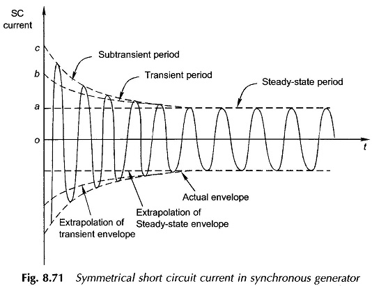
Iterative_waveform(I,:) = ((Vq1/xd)+(((Vq1/xDd)-(Vq1/xd))*exp(-t1/TDd))+(((Vq1/xDDd)-(Vq1/xDd))*exp(-t1/TDDd))).*sin(2*pi*f1*t1);

(This is the short current waveform of a synchrounous machine)

Vq1 = 556

t1 = known

xd = unknown

xDd = unknown

TDd = unknown

TDDd = unknown

xDDd = unknown

Problem:

1. The curvefit tool cannot curvefit the waveform even with the equation therefore I am trying to produce an iterative method to produce the correct variables
2. Using an r^2 value on a sine wave is inaccurate, due to the fact that a perfect waveform could be out of phase from the original data. I can't find an error checking method for accrurately producing a error.

Question:

1. does anyone know of a robust error checking method for a sinewave (was thinking of abs() then using r^2)
2. does know how to converge using an error method for a sine wave due to the r^2 values increasing and decreasing through all iterations

Answer 1

[David Wilson]

Here's my attempt at fitting uusing lsqcurvefit from the optimisation toolbox.

First I generate some synthetic data to subsequently fit that follows your curve (since you didn't think to give us any)

Vq1 = 556; % known constant
N = 200; % # of points 
t = linspace(0,0.2,N)'; 
f = 50; % presumably 50 Hz. 

% Set values for constants 
xd = 1;
xDd = 2;
TDd = 0.1;
TDDd = 0.05;
xDDd = 0.3; 
phi = -0.6; % initial phase offset 

y = (Vq1/xd+((Vq1/xDd-Vq1/xd))*exp(-t/TDd)  + ... 
    (((Vq1/xDDd)-(Vq1/xDd))*exp(-t/TDDd))).* ... 
    sin(2*pi*f*t+phi);

plot(t,y,'.-')

Now we are ready to do the fitting:

%% Now use lsqcurvefit 
p0 = 3*[1,1,1,  1,   1,    1]'; % guess of parameters 
LB =   [0,0,0,  0,   0,   -5]'; % can put anything here, even -inf. 
UB = 10*[1,1,1,  1,   1,    1]'; 

fun = @(p, t) (Vq1/p(1)+((Vq1/p(2)-Vq1/p(1)))*exp(-t/p(3))  + ... 
              (((Vq1/p(5))-(Vq1/p(2)))*exp(-t/p(4)))).* ... 
               sin(2*pi*f*t+p(6));
pfit = lsqcurvefit(fun,p0,... 
                t,y, ... 
                LB,UB)

yfit = fun(pfit,t); 
plot(t,y,'r.', t,yfit,'b-'); 

We get a pretty good fit since I start reasonably near the values used to generate the original curve.

[Harry Bumfrey]

Thanks, yeh sorry unfortuantly im unable to give physical data information due to company confidentiality.