Crack Identification from Accelerometer Data

This example shows how to use wavelet and deep learning techniques to detect transverse pavement cracks and localize their position. The example demonstrates the use of wavelet scattering sequences as inputs to a gated recurrent unit (GRU) and 1-D convolutional network to classify time series based on the presence or absence of a crack. The data are vertical acceleration measurements obtained from a sensor mounted on the suspension knuckle of the front passenger seat wheel. Early identification of developing transverse cracks is important for pavement performance evaluation and maintenance. Reliable automatic detection methods enable more frequent and extensive monitoring.

Please read the Data - Description and Required Attributions before running this example. All data import and preprocessing is described in the Data — Download and Import and the Data — Preprocessing sections. If you want to skip the training-test set creation, preprocessing, feature extraction, and model training, you can go directly to the Classification and Analysis section. There you can load the preprocessed test data as well as the extracted features and trained models.

Data — Description and Required Attributions

The data used in this example was retrieved from the Mendeley Data open data repository [2]. The data is distributed under a Creative Commons (CC) BY 4.0 license. Download the data and models used in this example in your temporary directory specified by MATLAB® tempdir command. If you choose to download the data in a folder different from tempdir, change the directory name in the subsequent instructions. Unzip the data into a folder specified as TransverseCrackData.

dataURL = "https://ssd.mathworks.com/supportfiles/wavelet/crackDetection/transverse_crack.zip";
saveFolder = fullfile(tempdir,"TransverseCrackData"); 
zipFile = fullfile(tempdir,"transverse_crack.zip");
websave(zipFile,dataURL);
unzip(zipFile,saveFolder)

After you unzip the data, the TransverseCrackData folder contains a subfolder called transverse_crack_latest. All subsequent commands must be run in this folder, or you can place this folder on the matlabpath.

The text file, vehiclevibrationdata.rights, included in the zip file contains the text of the CC BY 4.0 license. The data has been repackaged from the original Excel format into MAT-files.

Data acquisition is described in detail in [1]. Twelve four meter long sections of asphalt containing a centrally-located transverse crack and twelve equal-length uncracked sections were used. The data is obtained from three separate roads. The transverse cracks ranged in width from 2-13 mm with crack spacings from 7-35 mm. The sections were driven at three different speeds: 30 km/hr, 40 km/hr, and 50 km/hr. Vertical acceleration measurements from the front passenger suspension knuckle are acquired at a sampling frequency of 1.28 kHz. The speeds of 30, 40, and 50 km/hr correspond to sensor measurements every 6.5 mm at 30 km/hr, 8.68 mm at 40 km/hr, and 10.85 mm at 50 km/hr. See [1] for a detailed wavelet analysis of these data distinct from the analyses in this example.

In keeping with the stipulations of the CC BY 4.0 license, we note that the speed information of the original data is not retained in the data used in this example. The speed and road information are retained in the road1.mat, road2.mat, and road3.mat data files included in the data folder for completeness.

Data — Download and Import

Load the accelerometer data and their corresponding labels. There are 327 accelerometer recordings.

load(fullfile(saveFolder,"transverse_crack_latest","allroadData.mat"))
load(fullfile(saveFolder,"transverse_crack_latest","allroadLabel.mat"))

Data — Preprocessing

Obtain the length of all the time series. Display a bar graph of the number of time series per length.

tslen = cellfun(@length,allroadData);
uLen = unique(tslen);
Ng = histcounts(tslen);
Ng = Ng(Ng > 0);
bar(uLen,Ng,0.5)
grid on
AX = gca;
AX.YLim = [0 max(Ng)+15];
text(uLen(1),Ng(1)+10,num2str(Ng(1)))
text(uLen(2),Ng(2)+10,num2str(Ng(2)))
text(uLen(3),Ng(3)+10,num2str(Ng(3)))
xlabel("Length in Samples")
ylabel("Number of Series")
title("Time Series Length")

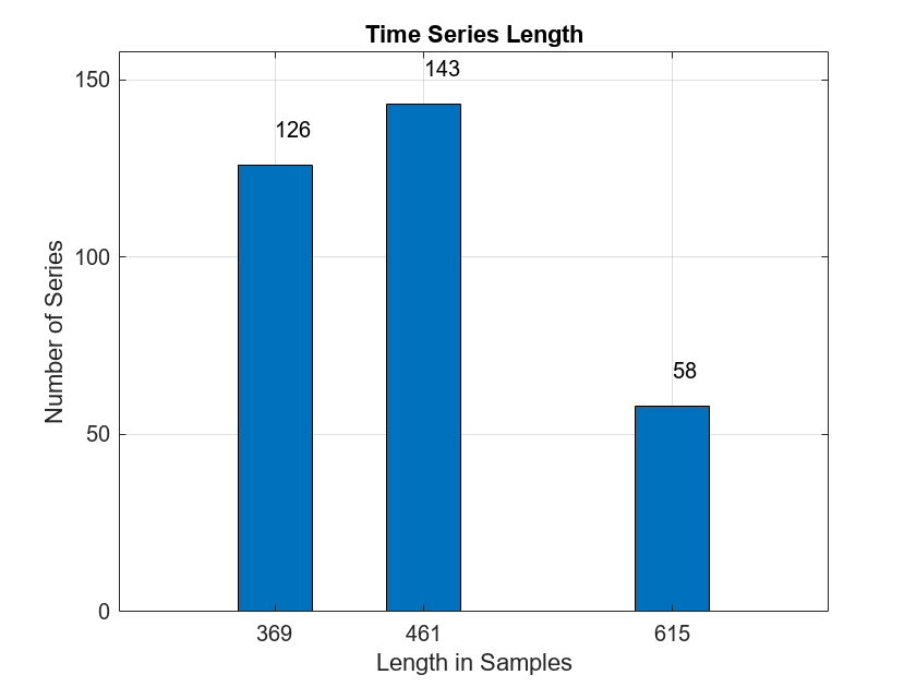
There are three unique lengths in the data set: 369, 461, and 615 samples. The vehicle is traveling at three different speeds but the distance traversed and sample rate is constant resulting in different data record lengths. Determine how many records are in the "Cracked" (CR) and "Uncracked" (UNCR) classes.

countlabels(allroadLabel)

ans=2×3 table
    Label    Count    Percent
    _____    _____    _______

    CR        109     33.333 
    UNCR      218     66.667 

This data set is significantly imbalanced. There are twice as many time series without a crack (UNCR) as series containing a crack (CR). This means that a classifier which predicts "Uncracked" on each record would achieve an accuracy of 67% without any learning.

The time series are also of different lengths. To use a wavelet scattering transform, a common input length is needed. In recurrent networks it is possible to use unequal length time series as inputs, but all time series in a mini-batch are padded or truncated based on the training options. This requires care in creating mini-batches for both training and testing to ensure the proper distribution of padded sequences. Further, it requires that you do not shuffle the data during training. With this small data set, shuffling the training data for each epoch is desirable. Accordingly, a common time series length is used.

The most common length is 461 samples. Further, the crack, if present, is centrally located in the recording. Accordingly, we can symmetrically extend the series with 369 samples to length 461 by reflecting the initial and final 46 samples. In the recordings with 615 samples, remove the initial 77 and final 77 samples.

Training — Feature Extraction and Network Training

The following sections generate the training and test sets, create the wavelet scattering sequences, and train both gated recurrent unit (GRU) and 1-D convolutional networks. First, extend or truncate the time series in both sets to obtain a common length of 461 samples.

allroadData = equalLenTS(allroadData);
all(cellfun(@numel,allroadData)== 461)

ans = logical
   1

Now each time series in both the cracked and uncracked data sets has 461 samples. Split the data in a training set consisting of 80% of the time series in each class and hold out the remaining 20% of each class for testing. Verify that the unbalanced proportions are retained in each set.

splt8020 = splitlabels(allroadLabel,0.80);
countlabels(allroadLabel(splt8020{1}))

ans=2×3 table
    Label    Count    Percent
    _____    _____    _______

    CR         87     33.333 
    UNCR      174     66.667 

countlabels(allroadLabel(splt8020{2}))

ans=2×3 table
    Label    Count    Percent
    _____    _____    _______

    CR        22      33.333 
    UNCR      44      66.667 

Create the training and test sets.

TrainData = allroadData(splt8020{1});
TrainLabels = allroadLabel(splt8020{1});
TestData = allroadData(splt8020{2});
TestLabels = allroadLabel(splt8020{2});

Shuffle the data and labels once before training.

idxS = randperm(length(TrainData));
TrainData = TrainData(idxS);
TrainLabels = TrainLabels(idxS);
idxS = randperm(length(TrainData));
TrainData = TrainData(idxS);
TrainLabels = TrainLabels(idxS);

Compute the scattering sequences for each of the training series. The scattering sequences are stored in a cell array to be compatible with the GRU and 1-D convolutional networks.

XTrainSCAT = cell(size(TrainData));
for kk = 1:numel(TrainData)
    XTrainSCAT{kk} = helperscat(TrainData{kk});
end
npaths = cellfun(@(x)size(x,1),XTrainSCAT);
inputSize = npaths(1);

Training — GRU Network

Construct the GRU network layers. Use two GRU layers with 30 hidden units each as well as two dropout layers. The input size is the number of scattering paths. To train this network on the raw time series, change the inputSize to 1 and transpose each time series to a row vector (1-by-461). If you want to skip the network training, you may go directly to the Classification and Analysis section. There you can load the trained GRU network as well as the preprocessed training and test sets.

numHiddenUnits1 = 30;
numHiddenUnits2 = 30;
numClasses = 2;
classFrequencies = countcats(allroadLabel);
Nsamp = sum(classFrequencies);
weightCR = 1/classFrequencies(1)*Nsamp/2;
weightUNCR = 1/classFrequencies(2)*Nsamp/2;
GRUlayers = [ ...
    sequenceInputLayer(inputSize,Name="InputLayer", ...
    Normalization="zerocenter")
    gruLayer(numHiddenUnits1,Name="GRU1",OutputMode="sequence")
    dropoutLayer(0.35,Name="Dropout1")
    gruLayer(numHiddenUnits2,Name="GRU2",OutputMode="last")
    dropoutLayer(0.2,Name="Dropout2")
    fullyConnectedLayer(numClasses,Name="FullyConnected")
    softmaxLayer(Name="smax");
    ];

classNames = ["CR" "UNCR"];

Because the classes are significantly unbalanced, use a weighted classification loss with the class weights proportional to the inverse class frequencies. Create a custom loss function that takes predictions Y and targets T and returns the weighted cross-entropy loss.

lossFcn = @(Y,T) crossentropy(Y,T,[weightCR weightUNCR], ...
    NormalizationFactor="all-elements", ...
    WeightsFormat="C")*numClasses;

Specify the training options. Choosing among the options requires empirical analysis. Because the training data has sequences with rows and columns corresponding to channels and time steps, respectively, specify the input data format "CTB" (channel, time, batch).

maxEpochs = 150;
miniBatchSize = 100;
options = trainingOptions("adam", ...
    L2Regularization=1e-3, ...
    MaxEpochs=maxEpochs, ...
    MiniBatchSize=miniBatchSize, ...
    Shuffle="every-epoch", ...
    Verbose=true, ...
    Plots="none", ...
    Metrics="accuracy", ...
    InputDataFormats="CTB");

Train the GRU network using the trainnet (Deep Learning Toolbox) function. For weighted classification, use the custom cross-entropy function. By default, the trainnet function uses a GPU if one is available. Training on a GPU requires a Parallel Computing Toolbox™ license and a supported GPU device. For information on supported devices, see GPU Computing Requirements (Parallel Computing Toolbox). Otherwise, the trainnet function uses the CPU. To specify the execution environment, use the ExecutionEnvironment training option

[scatGRUnet,infoGRU] = trainnet(XTrainSCAT,TrainLabels,GRUlayers,lossFcn,options);

    Iteration    Epoch    TimeElapsed    LearnRate    TrainingLoss    TrainingAccuracy
    _________    _____    ___________    _________    ____________    ________________
            1        1       00:00:08        0.001          0.6866                  60
           50       25       00:00:15        0.001         0.68871                  54
          100       50       00:00:17        0.001         0.24968                  93
          150       75       00:00:19        0.001         0.10168                  97
          200      100       00:00:21        0.001        0.065607                  99
          250      125       00:00:23        0.001        0.046649                  99
          300      150       00:00:25        0.001        0.020625                 100
Training stopped: Max epochs completed

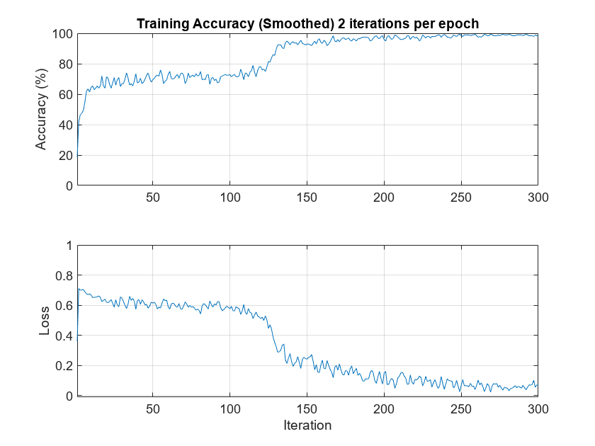
Plot the smoothed training accuracy and loss per iteration.

iterPerEpoch = floor(length(XTrainSCAT)/miniBatchSize);
figure
tiledlayout(2,1)
nexttile
smoothedACC = filter(1/iterPerEpoch*ones(iterPerEpoch,1),1, ...
    infoGRU.TrainingHistory.Accuracy);
smoothedLoss = filter(1/iterPerEpoch*ones(iterPerEpoch,1),1, ...
    infoGRU.TrainingHistory.Loss);
plot(smoothedACC)
title("Training Accuracy (Smoothed) "+ ...
    num2str(iterPerEpoch)+" Iterations per Epoch")
ylabel("Accuracy (%)")
ylim([0 100.1])
grid on
xlim([1 length(smoothedACC)])
nexttile
plot(smoothedLoss)
ylim([-0.01 1])
grid on
xlim([1 length(smoothedLoss)])
ylabel("Loss")
xlabel("Iteration")

Obtain the wavelet scattering transforms of the held-out test data for classification.

XTestSCAT = cell(size(TestData));
for kk = 1:numel(TestData)
    XTestSCAT{kk} = helperscat(TestData{kk});
end

Training — 1-D Convolutional Network

Train a 1-D convolutional network with wavelet scattering sequences. If you want to skip the network training, you may go directly to the Classification and Analysis section. There you can load the trained convolutional network as well as the preprocessed training and test sets.

Construct and train the 1-D convolutional network. There are 28 paths in the scattering network.

conv1dLayers = [
    sequenceInputLayer(28,MinLength=58,Normalization="zerocenter")
    convolution1dLayer(3,24,Stride=2)
    batchNormalizationLayer
    reluLayer
    maxPooling1dLayer(4)
    convolution1dLayer(3,16,Padding="same")
    batchNormalizationLayer
    reluLayer
    maxPooling1dLayer(2)
    fullyConnectedLayer(150)
    fullyConnectedLayer(2)
    globalAveragePooling1dLayer
    softmaxLayer
    ];

convoptions = trainingOptions("adam", ...
    InitialLearnRate=0.01, ...
    LearnRateSchedule="piecewise", ...
    LearnRateDropFactor=0.5, ...
    LearnRateDropPeriod=5, ...
    MaxEpochs=50, ...
    Verbose=true, ...
    Plots="none", ...
    Metrics="accuracy", ...
    MiniBatchSize=miniBatchSize, ...
    InputDataFormats="CTB");

[scatCONV1Dnet,infoCONV] = ...
    trainnet(XTrainSCAT,TrainLabels,conv1dLayers,lossFcn,convoptions);

    Iteration    Epoch    TimeElapsed    LearnRate    TrainingLoss    TrainingAccuracy
    _________    _____    ___________    _________    ____________    ________________
            1        1       00:00:03         0.01         0.67389                  34
           50       25       00:00:06     0.000625        0.012259                 100
          100       50       00:00:09   1.9531e-05        0.010495                 100
Training stopped: Max epochs completed

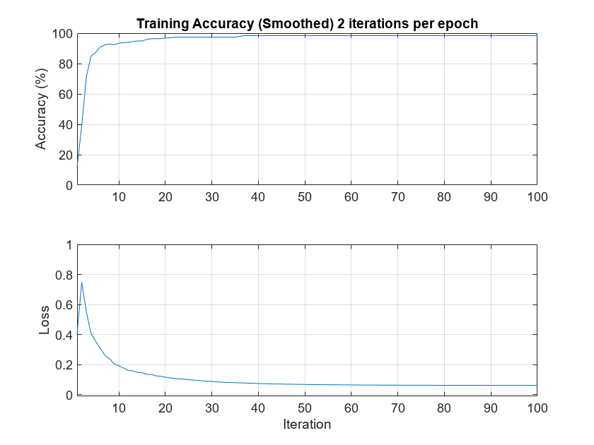
Plot the smoothed training accuracy and loss per iteration.

iterPerEpoch = floor(length(XTrainSCAT)/miniBatchSize);
figure
tiledlayout(2,1)
nexttile
smoothedACC = filter(1/iterPerEpoch*ones(iterPerEpoch,1),1, ...
    infoCONV.TrainingHistory.Accuracy);
smoothedLoss = filter(1/iterPerEpoch*ones(iterPerEpoch,1),1, ...
    infoCONV.TrainingHistory.Loss);
plot(smoothedACC)
title("Training Accuracy (Smoothed) "+ ...
    num2str(iterPerEpoch)+" Iterations per Epoch")
ylabel("Accuracy (%)")
ylim([0 100.1])
grid on
xlim([1 length(smoothedACC)])
nexttile
plot(smoothedLoss)
ylim([-0.01 1])
grid on
xlim([1 length(smoothedLoss)])
ylabel("Loss")
xlabel("Iteration")

Classification and Analysis

Load the trained gated recurrent unit (GRU) and 1-D convolutional networks along with the test data and scattering sequences. All data, features, and networks were created in the Training — Feature Extraction and Network Training section.

load(fullfile(saveFolder,"transverse_crack_latest","TestData.mat"))
load(fullfile(saveFolder,"transverse_crack_latest","TestLabels.mat"))
load(fullfile(saveFolder,"transverse_crack_latest","XTestSCAT.mat"))
load(fullfile(saveFolder,"transverse_crack_latest","scatGRUnet.mat"))
scatGRUnet = dag2dlnetwork(scatGRUnet);
load(fullfile(saveFolder,"transverse_crack_latest","scatCONV1Dnet.mat"))
scatCONV1Dnet = dag2dlnetwork(scatCONV1Dnet);

If you additionally want the preprocessed data, labels, and wavelet scattering sequences for the training data, you can load those with the following commands. These data and labels are not used in the remainder of this example if you want to skip the following load commands.

load(fullfile(saveFolder,"transverse_crack_latest","TrainData.mat"))
load(fullfile(saveFolder,"transverse_crack_latest","TrainLabels.mat"))
load(fullfile(saveFolder,"transverse_crack_latest","XTrainSCAT.mat"))

Examine the number of time series per class in the test set. Note the test set is significantly imbalanced as discussed in Data — Preprocessing section.

countlabels(TestLabels)

ans=2×3 table
    Label    Count    Percent
    _____    _____    _______

    CR        22      33.333 
    UNCR      44      66.667 

XTestSCAT contains the wavelet scattering sequences computed for the raw time series in TestData.

Show the GRU model performance on the test data not used in model training.

miniBatchSize = 15;
scores = minibatchpredict(scatGRUnet,XTestSCAT, ...
    MiniBatchSize=miniBatchSize, ...
    InputDataFormats="CTB");
ypredSCAT = scores2label(scores,classNames);
figure
confusionchart(TestLabels,ypredSCAT,RowSummary="row-normalized", ...
    ColumnSummary="column-normalized")
title({"GRU Network — Wavelet Scattering Sequences"; ...
    "Confusion Chart with Precision and Recall"})

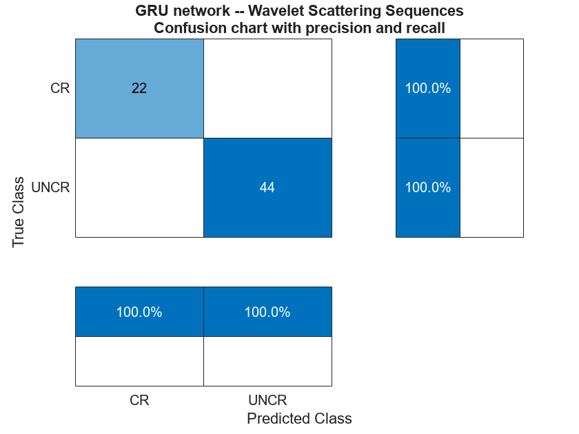
In spite of the large imbalance in the classes and the small data set, the precision and recall values indicate the network performs well on the test data. Specifically, the precision and recall values for "Cracked" data are excellent. This is achieved in spite of the fact that 67% of the records in the training set were "Uncracked". The network has not overlearned to classify the time series as "Uncracked" in spite of the imbalance.

If you set inputSize = 1 and transpose the time series in the training data, you can retrain the GRU network on the raw time series data. This was done on the same data in the training set. You can load that network and check the performance on the test set.

load(fullfile(saveFolder,"transverse_crack_latest","tsGRUnet.mat"))
tsGRUnet = dag2dlnetwork(tsGRUnet);
rawTest = cellfun(@transpose,TestData,UniformOutput=false);
miniBatchSize = 15;
scores = minibatchpredict(tsGRUnet,rawTest, ...
    MiniBatchSize=miniBatchSize, ...
    InputDataFormats="CTB");
YPredraw = scores2label(scores,classNames);

confusionchart(TestLabels,YPredraw,RowSummary="row-normalized", ...
    ColumnSummary="column-normalized")
title({"GRU Network — Raw Time Series"; ...
    "Confusion Chart with Precision and Recall"})

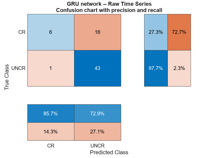
For this network, the performance is not good. Specifically, the recall for the "Cracked" data is poor. The number of false negatives for the "Cracked" data is quite large. This is exactly what you would expect with an imbalanced data set when the model has not learned well.

Test the 1-D convolutional network trained with the wavelet scattering sequences.

miniBatchSize = 15;
scores = minibatchpredict(scatCONV1Dnet,XTestSCAT, ...
    MiniBatchSize=miniBatchSize, ...
    InputDataFormats="CTB");
YPredSCAT = scores2label(scores,classNames);
figure
confusionchart(TestLabels,YPredSCAT,RowSummary="row-normalized", ...
    ColumnSummary="column-normalized")
title({"1-D Convolutional Network — Wavelet Scattering Sequences"; ...
    "Confusion Chart with Precision and Recall"})

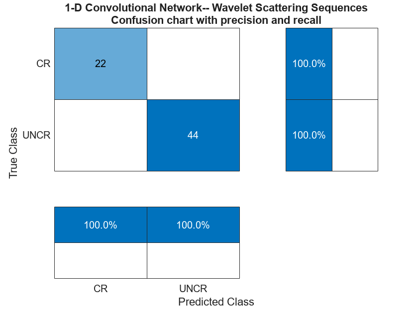
The performance of the convolutional network with scattering sequences is excellent and is consistent with the performance of the GRU network. Precision and recall on the minority class demonstrate robust learning.

To train the 1-D convolutional network on the raw sequences, set inputSize to 1 in the sequenceInputLayer. Set MinLength to 461. You can load and test that network trained using the same data and same network architecture.

load(fullfile(saveFolder,"transverse_crack_latest","tsCONV1Dnet.mat"))
tsCONV1Dnet = dag2dlnetwork(tsCONV1Dnet);
miniBatchSize = 15;
TestDataT = cellfun(@transpose,TestData,UniformOutput=false);
socres = minibatchpredict(tsCONV1Dnet,TestDataT, ...
    MiniBatchSize=miniBatchSize, ...
    InputDataFormats="CTB");
YPredRAW = scores2label(socres,classNames);
confusionchart(TestLabels,YPredRAW,RowSummary="row-normalized", ...
    ColumnSummary="column-normalized")
title({"1-D Convolutional Network — Raw Sequences"; ...
    "Confusion Chart with Precision and Recall"})

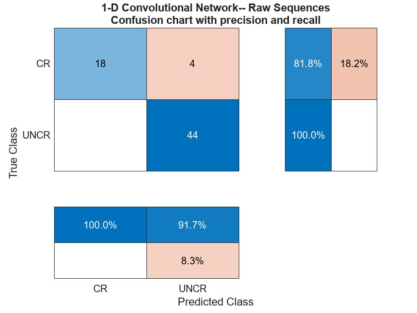
The 1-D convolution network with the raw sequences performs well but not quite as well as the convolutional network trained with the wavelet scattering sequences.

Wavelet Inference and Analysis

This section demonstrates how to classify a single time series using wavelet analysis with a pretrained model. The model used is the 1-D convolutional network trained on wavelet scattering sequences. Load the trained network and some test data if you have not already loaded these in the previous section.

load(fullfile(saveFolder,"transverse_crack_latest","scatCONV1Dnet.mat"))
scatCONV1Dnet = dag2dlnetwork(scatCONV1Dnet);
load(fullfile(saveFolder,"transverse_crack_latest","TestData.mat"))

Construct the wavelet scattering network to transform the data. Select a time series from the test data and classify the data. If the model classifies the time series as "Cracked", investigate the series for the position of the crack in the waveform.

sf = waveletScattering(SignalLength=461, ...
    OversamplingFactor=1,QualityFactors=[8 1], ...
    InvarianceScale=0.05,Boundary="reflection",SamplingFrequency=1280);
idx = 22;
data = TestData{idx};
[smat,x] = featureVectors(data,sf);
scores = minibatchpredict(scatCONV1Dnet,smat,InputDataFormats="CTB");
PredictedClass = scores2label(scores,classNames);
if isequal(PredictedClass,"CR") 
    fprintf("Crack detected. Computing wavelet transform modulus maxima.\n")
    wtmm(data,Scaling="local")
end

Crack detected. Computing wavelet transform modulus maxima.

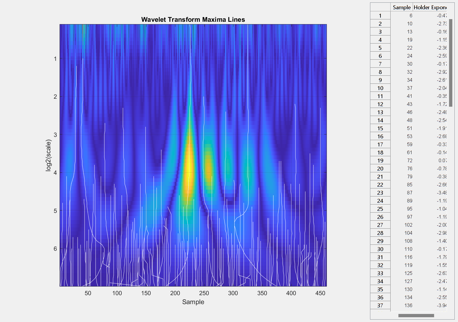
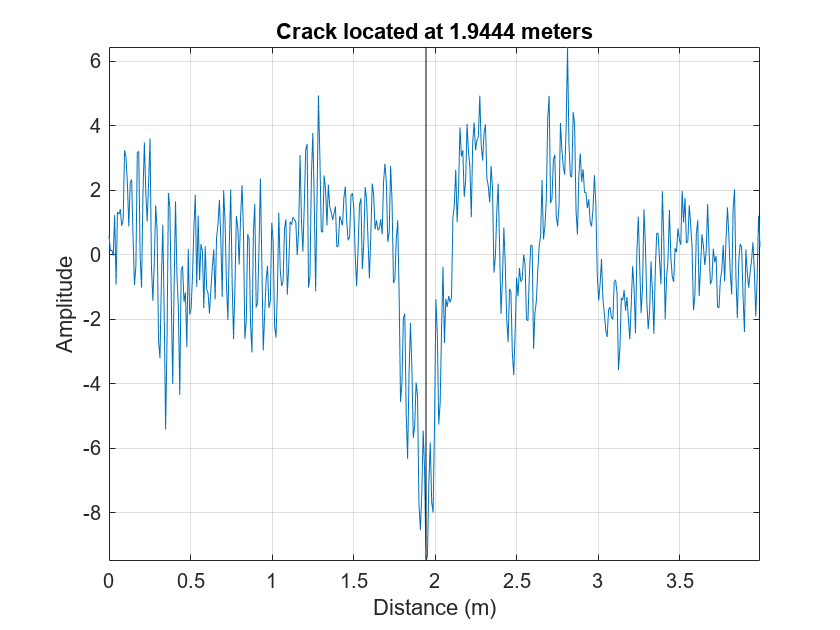
The wavelet transform modulus maxima (WTMM) technique shows a maxima line converging to the finest scale at sample 225. Maxima lines that converge to fine scales are a good estimate of where singularities are in a time series. This makes sample 225 a good estimate of the location of the crack.

figure
plot(x,data)
axis tight
hold on
plot([x(225) x(225)],[min(data) max(data)],"k")
hold off
grid on
title("Crack Located at "+num2str(x(225))+" Meters")
xlabel("Distance (m)")
ylabel("Amplitude")

You can increase your confidence in this location by using multiresolution analysis (MRA) techniques and identifying changes in slope in long-scale wavelet MRA series. See Practical Introduction to Multiresolution Analysis for an introduction to MRA techniques. In [1] the difference in energy between "Cracked" and "Uncracked" series occurred in the low frequency bands, specifically in the interval of [10,20] Hz. Accordingly, the following MRA is focused on signal components in the frequency bands from [10,80] Hz. In these bands, identify linear changes in the data. Plot the change points along with the MRA components.

[mra,chngpts] = helperMRA(data,x);

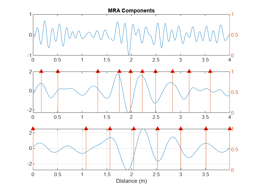
The MRA-based changepoint analysis has helped to confirm the WTMM analysis in identifying the region around 1.94 meters as the probable location of the crack.

Summary

This example showed how to use wavelet scattering sequences with both recurrent and convolutional networks to classify time series. The example further demonstrated how wavelet techniques can help to localize features on the same spatial (time) scale as the original data.

References

[1] Yang, Qun and Shishi Zhou. "Identification of asphalt pavement transverse cracking based on vehicle vibration signal analysis.", Road Materials and Pavement Design, 2020, 1-19. https://doi.org/10.1080/14680629.2020.1714699.

[2] Zhou,Shishi. "Vehicle vibration data." https://data.mendeley.com/datasets/3dvpjy4m22/1. Data is used under CC BY 4.0. Data is repackaged from original Excel data format to MAT-files. Speed label removed and only "crack" or "nocrack" label retained.

Appendix

Helper functions used in this example.

function smat = helperscat(datain)
% This helper function is only in support of Wavelet Toolbox examples.
% It may change or be removed in a future release.
datain = single(datain);

sn = waveletScattering(SignalLength=length(datain), ...
    OversamplingFactor=1,QualityFactors=[8 1], ...
    InvarianceScale=0.05,Boundary="reflection",SamplingFrequency=1280);
smat = sn.featureMatrix(datain);

end

%-----------------------------------------------------------------------
function dataUL = equalLenTS(data)
% This function in only in support of Wavelet Toolbox examples.
% It may change or be removed in a future release.
N = length(data);
dataUL = cell(N,1);
for kk = 1:N
    L = length(data{kk});
    switch L
        case 461
            dataUL{kk} = data{kk};
        case 369
            Ndiff = 461-369;
            pad = Ndiff/2;
            dataUL{kk} = [flip(data{kk}(1:pad)); data{kk} ; ...
                flip(data{kk}(L-pad+1:L))];     
        otherwise
            Ndiff = L-461;
            zrs = Ndiff/2;
            dataUL{kk} = data{kk}(zrs:end-zrs-1);
    end
end       

end

%--------------------------------------------------------------------------
function [fmat,x] = featureVectors(data,sf)
% This function is only in support of Wavelet Toolbox examples.
% It may change or be removed in a future release.
data = single(data);
N = length(data);
dt = 1/1280;
if N < 461
    Ndiff = 461-N;
    pad = Ndiff/2;
    dataUL = [flip(data(1:pad)); data ; ...
                flip(data(N-pad+1:N))];   
     rate = 5e4/3600;
     dx = rate*dt;
     x = 0:dx:(N*dx)-dx;     
elseif N > 461
    Ndiff = N-461;
    zrs = Ndiff/2;
    dataUL = data(zrs:end-zrs-1);
    rate = 3e4/3600;
    dx = rate*dt;
    x = 0:dx:(N*dx)-dx;
else
    dataUL = data;
    rate = 4e4/3600;
    dx = rate*dt;
    x = 0:dx:(N*dx)-dx;
end
fmat = sf.featureMatrix(dataUL);
end

%------------------------------------------------------------------------------
function [mra,chngpts] = helperMRA(data,x)
% This function is only in support of Wavelet Toolbox examples.
% It may change or be removed in a future release.
mra = modwtmra(modwt(data,"sym3"),"sym3");
mraLev = mra(4:6,:);
Ns = size(mraLev,1);
thresh = [2, 4, 8];
chngpts = false(size(mraLev));
% Determine changepoints. We want different thresholds for different
% resolution levels.
for ii = 1:Ns
    chngpts(ii,:) = ischange(mraLev(ii,:),"linear",2,Threshold=thresh(ii));
end
tiledlayout(Ns,1)
for kk = 1:Ns
    idx = double(chngpts(kk,:));
    idx(idx == 0) = NaN;    
    nexttile
    plot(x,mraLev(kk,:))
    if kk == 1
        title("MRA Components")
    end
    yyaxis right
    hs = stem(x,idx);
    hs.ShowBaseLine="off";
    hs.Marker = "^";
    hs.MarkerFaceColor = [1 0 0];
end
grid on
axis tight
xlabel("Distance (m)")
end